Possible Analysis and Keywords

Regular Expressions
String Manipulation
Merging Datasets
Socioeconomic Data
Canadian Data
Regression
Housing

Goals

Find and extract socio-economic data from Statistics Canada. In this example we manipulate and plot unemployment rates and housing starts. Relationships between the two datasets are examined.

Data Provider

Statistics Canada hosts a large set of socio-economic datasets. When searching through these, take note of the table identifier. The cansim package provides an API for downloading these tables. See also the cansim vignette for examples and instructions to pull Statistics Canada datasets.

For larger tables, cansim offers sqlite integration. See for example the vignette

Installing cansim

There are a lot of specifics in the package vignette, one way to view them is to install the library and use the vignette function:

install.packages("cansim")
library(cansim)
vignette("cansim")

#code not run for this document.

Basic libraries

library(tidyverse) # for its nice flow.
library(cansim) #for pulling Stat Can socioeconomic data
library(lubridate) # for dealing with dates
library(GGally) # for pairs plot
library(ggpubr) # for putting a regression equation onto a ggplot figure

Pulling a table

Visit here for example to see labor force data in html. Notice that the StatCan webpage shows the table id, here it is table: 14-10-0287-01.

We’ll use that to grab the table. Be warned that this data table is a csv of around 1 GB in size. While we’re at it, let’s remake some column names to make them more R friendly.

data = get_cansim("14-10-0287-01") |> rename_all(make.names) 

data |> glimpse()

## Rows: 4,927,068
## Columns: 33
## $ REF_DATE                                             <chr> "1976-01", "1976-…
## $ GEO                                                  <chr> "Canada", "Canada…
## $ DGUID                                                <chr> "2016A000011124",…
## $ UOM                                                  <chr> "Persons", "Perso…
## $ UOM_ID                                               <chr> "249", "249", "24…
## $ SCALAR_FACTOR                                        <chr> "thousands", "tho…
## $ SCALAR_ID                                            <chr> "3", "3", "3", "3…
## $ VECTOR                                               <chr> "v2062809", "v206…
## $ COORDINATE                                           <chr> "1.1.1.1.1.1", "1…
## $ VALUE                                                <dbl> 16852.4, 16852.4,…
## $ STATUS                                               <chr> NA, NA, NA, NA, N…
## $ SYMBOL                                               <chr> NA, NA, NA, NA, N…
## $ TERMINATED                                           <chr> NA, NA, NA, NA, N…
## $ DECIMALS                                             <chr> "1", "1", "1", "1…
## $ GeoUID                                               <chr> "11124", "11124",…
## $ Hierarchy.for.GEO                                    <chr> "1", "1", "1", "1…
## $ Classification.Code.for.Labour.force.characteristics <chr> NA, NA, NA, NA, N…
## $ Hierarchy.for.Labour.force.characteristics           <chr> "1", "1", "1", "1…
## $ Classification.Code.for.Sex                          <chr> NA, NA, NA, NA, N…
## $ Hierarchy.for.Sex                                    <chr> "1", "1", "1", "1…
## $ Classification.Code.for.Age.group                    <chr> NA, NA, NA, NA, N…
## $ Hierarchy.for.Age.group                              <chr> "1", "1", "8", "8…
## $ Classification.Code.for.Statistics                   <chr> NA, NA, NA, NA, N…
## $ Hierarchy.for.Statistics                             <chr> "1", "1", "1", "1…
## $ Classification.Code.for.Data.type                    <chr> NA, NA, NA, NA, N…
## $ Hierarchy.for.Data.type                              <chr> "1", "2", "1", "2…
## $ val_norm                                             <dbl> 16852400, 1685240…
## $ Date                                                 <date> 1976-01-01, 1976…
## $ Labour.force.characteristics                         <fct> Population, Popul…
## $ Sex                                                  <fct> Both sexes, Both …
## $ Age.group                                            <fct> 15 years and over…
## $ Statistics                                           <fct> Estimate, Estimat…
## $ Data.type                                            <fct> Seasonally adjust…

There are nearly 5 million rows of data!

Make a few plots of Employment statistics

Stat Can tables are structured so that each row has a single value and columns define attributes about that value Each row of data has a specific attribute sex, age (Age.group), and Location (GEO) attributes, for units of the value (SCALAR_FACTOR), the specific type of labour force characteristic measured (Labour.force.characteristics), and the differences data types such as point estimates and (bootstrap) standard errors (Statistics), and raw or seasonally adjusted (Data.type). In general this means that we need to filter and reshape the data.

Let’s inventory a few of these columns so that the exact spelling of attributes can be used below in the plots.

data$Labour.force.characteristics  |> unique()

## [1] Population           Labour force         Employment          
## [4] Full-time employment Part-time employment Unemployment        
## [7] Unemployment rate    Participation rate   Employment rate     
## 9 Levels: Population Labour force Employment ... Employment rate

data$Statistics  |> unique()

## [1] Estimate                               
## [2] Standard error of estimate             
## [3] Standard error of month-to-month change
## [4] Standard error of year-over-year change
## 4 Levels: Estimate ... Standard error of year-over-year change

data$Age.group  |> unique()

## [1] 15 years and over 15 to 64 years    15 to 24 years    15 to 19 years   
## [5] 20 to 24 years    25 years and over 25 to 54 years    55 years and over
## [9] 55 to 64 years   
## 9 Levels: 15 years and over 15 to 24 years 15 to 19 years ... 55 to 64 years

data$GEO  |> unique()

##  [1] "Canada"                    "Newfoundland and Labrador"
##  [3] "Prince Edward Island"      "Nova Scotia"              
##  [5] "New Brunswick"             "Quebec"                   
##  [7] "Ontario"                   "Manitoba"                 
##  [9] "Saskatchewan"              "Alberta"                  
## [11] "British Columbia"

Plotting provinces against each other

Let’s consider provincial differences in employment rate for 25-55 year olds. Using the spelling from the above output we can set up the data filters.

When pivot_wider Works, But Not As Intended; Common Errors and How to Fix Them

Pivoting a data table will spread out a variable into new columns. Sometimes it’s more convenient to have each province as it’s own column. Here we do this to plot provinces against each other and see how they relate. It can be helpful to see how to accidentally break things, so let’s start there.
I will need to filter the data so let’s start there. Here we go right from selecting columns, filtering and then pivoting wider, which will help when plotting. Take a look at the output.

data |> select(GEO,Sex,Age.group,Labour.force.characteristics,REF_DATE,VALUE)|>
  filter(Sex == "Both sexes") |> 
  filter(GEO != "Canada")|> # since the Canada value will be a type of weighted average
  filter( Labour.force.characteristics == "Unemployment rate")|>
  filter(Age.group == "25 to 54 years")|>
  pivot_wider(names_from= GEO, values_from=VALUE) |>  # puts each province into its own column
  rename_all(make.names) # rebuilt the province names

## Warning: Values are not uniquely identified; output will contain list-cols.
## * Use `values_fn = list` to suppress this warning.
## * Use `values_fn = length` to identify where the duplicates arise
## * Use `values_fn = {summary_fun}` to summarise duplicates

## # A tibble: 548 × 14
##    Sex        Age.group Labour.force.ch… REF_DATE Newfoundland.an… Prince.Edward.I…
##    <fct>      <fct>     <fct>            <chr>    <list>           <list>          
##  1 Both sexes 25 to 54… Unemployment ra… 1976-01  <dbl [5]>        <dbl [5]>       
##  2 Both sexes 25 to 54… Unemployment ra… 1976-02  <dbl [5]>        <dbl [5]>       
##  3 Both sexes 25 to 54… Unemployment ra… 1976-03  <dbl [5]>        <dbl [5]>       
##  4 Both sexes 25 to 54… Unemployment ra… 1976-04  <dbl [5]>        <dbl [5]>       
##  5 Both sexes 25 to 54… Unemployment ra… 1976-05  <dbl [5]>        <dbl [5]>       
##  6 Both sexes 25 to 54… Unemployment ra… 1976-06  <dbl [5]>        <dbl [5]>       
##  7 Both sexes 25 to 54… Unemployment ra… 1976-07  <dbl [5]>        <dbl [5]>       
##  8 Both sexes 25 to 54… Unemployment ra… 1976-08  <dbl [5]>        <dbl [5]>       
##  9 Both sexes 25 to 54… Unemployment ra… 1976-09  <dbl [5]>        <dbl [5]>       
## 10 Both sexes 25 to 54… Unemployment ra… 1976-10  <dbl [5]>        <dbl [5]>       
## # … with 538 more rows, and 8 more variables: Nova.Scotia <list>,
## #   New.Brunswick <list>, Quebec <list>, Ontario <list>, Manitoba <list>,
## #   Saskatchewan <list>, Alberta <list>, British.Columbia <list>

The provinces are now list variables, whereas they should be doubles (single numbers). It wasn’t obvious to me what went wrong the first time I broke a pivot table like this. Let’s re-run those steps without the pivot_wider and see if it helps to diagnose the root of the problem. This is one of the great parts of tidyverse, we just rerun a subset of the above code, or explicitely extract one of those list elements from the original call:

# run fewer lines of the previous code:
data |> select(GEO,Sex,Age.group,Labour.force.characteristics,REF_DATE,VALUE)|>
  filter(Sex == "Both sexes") |> 
  filter(GEO != "Canada")|> # since the Canada value will be a type of weighted average
  filter( Labour.force.characteristics == "Unemployment rate")|>
  filter(Age.group == "25 to 54 years")

## # A tibble: 27,400 × 6
##    GEO                       Sex    Age.group  Labour.force.char… REF_DATE VALUE
##    <chr>                     <fct>  <fct>      <fct>              <chr>    <dbl>
##  1 Newfoundland and Labrador Both … 25 to 54 … Unemployment rate  1976-01   10.1
##  2 Newfoundland and Labrador Both … 25 to 54 … Unemployment rate  1976-01   11.4
##  3 Newfoundland and Labrador Both … 25 to 54 … Unemployment rate  1976-01   NA  
##  4 Newfoundland and Labrador Both … 25 to 54 … Unemployment rate  1976-01   NA  
##  5 Newfoundland and Labrador Both … 25 to 54 … Unemployment rate  1976-01   NA  
##  6 Prince Edward Island      Both … 25 to 54 … Unemployment rate  1976-01    5.7
##  7 Prince Edward Island      Both … 25 to 54 … Unemployment rate  1976-01    7.3
##  8 Prince Edward Island      Both … 25 to 54 … Unemployment rate  1976-01   NA  
##  9 Prince Edward Island      Both … 25 to 54 … Unemployment rate  1976-01   NA  
## 10 Prince Edward Island      Both … 25 to 54 … Unemployment rate  1976-01   NA  
## # … with 27,390 more rows

## or view the problem this way, select Ontario and check out the first element:
# data |> select(GEO,Sex,Age.group,Labour.force.characteristics,REF_DATE,VALUE)|>
#   filter(Sex == "Both sexes") |> 
#   filter(GEO != "Canada")|> # since the Canada value will be a type of weighted average
#   filter( Labour.force.characteristics == "Unemployment rate")|>
#   filter(Age.group == "25 to 54 years")|>
#   pivot_wider(names_from= GEO, values_from=VALUE) |>  # puts each province into its own column
#   rename_all(make.names) |> 
#   select(Ontario)|> head|> .[[1]]

If you look closely at the output in the first strategy you’ll notice that there are multiple rows which only differ in their VALUE. This means that pivot_wider is mapping multiple rows of VALUE into a single element. R handles this by smashing all those values together into list elements.

In order to have a one-to-one mapping add another variable to create a unique mapping. Taking another close look at the glimpse output above, we can see that there is more than one Data.type. Checking out its values we see the following:

data$Data.type  |> unique()

## [1] Seasonally adjusted Unadjusted          Trend-cycle        
## Levels: Seasonally adjusted Unadjusted Trend-cycle

The multiple VALUEs are made unique when considering the Data.type variable. To simplify things, let’s select the Unadjusted unemployment rate.

When pivot_wider Works As Intended

data |> select(GEO,Sex,Age.group,Labour.force.characteristics,REF_DATE,VALUE,Data.type)|>
  filter(Sex == "Both sexes") |> 
  filter(GEO != "Canada")|> # since the Canada value will be a type of weighted average
  filter( Labour.force.characteristics == "Unemployment rate")|>
  filter(Age.group == "25 to 54 years")|>
  filter(Data.type == "Unadjusted")|>
  pivot_wider(names_from= GEO, values_from=VALUE) |>  # puts each province into its own column
  rename_all(make.names)

## # A tibble: 548 × 15
##    Sex        Age.group      Labour.force.ch… REF_DATE Data.type Newfoundland.an…
##    <fct>      <fct>          <fct>            <chr>    <fct>                <dbl>
##  1 Both sexes 25 to 54 years Unemployment ra… 1976-01  Unadjust…             11.4
##  2 Both sexes 25 to 54 years Unemployment ra… 1976-02  Unadjust…             12.3
##  3 Both sexes 25 to 54 years Unemployment ra… 1976-03  Unadjust…             11.7
##  4 Both sexes 25 to 54 years Unemployment ra… 1976-04  Unadjust…             13.2
##  5 Both sexes 25 to 54 years Unemployment ra… 1976-05  Unadjust…             12.1
##  6 Both sexes 25 to 54 years Unemployment ra… 1976-06  Unadjust…              9.6
##  7 Both sexes 25 to 54 years Unemployment ra… 1976-07  Unadjust…              9.9
##  8 Both sexes 25 to 54 years Unemployment ra… 1976-08  Unadjust…             10.2
##  9 Both sexes 25 to 54 years Unemployment ra… 1976-09  Unadjust…              8.3
## 10 Both sexes 25 to 54 years Unemployment ra… 1976-10  Unadjust…              9.2
## # … with 538 more rows, and 9 more variables: Prince.Edward.Island <dbl>,
## #   Nova.Scotia <dbl>, New.Brunswick <dbl>, Quebec <dbl>, Ontario <dbl>,
## #   Manitoba <dbl>, Saskatchewan <dbl>, Alberta <dbl>, British.Columbia <dbl>

Plotting Variables Against Each Other.

data |> select(GEO,Sex,Age.group,Labour.force.characteristics,REF_DATE,VALUE,Data.type)|>
  filter(Sex == "Both sexes") |> 
  filter(GEO != "Canada")|> # since the Canada value will be a type of weighted average
  filter( Labour.force.characteristics == "Unemployment rate")|>
  filter(Age.group == "25 to 54 years")|>
  filter(Data.type == "Unadjusted")|>
  pivot_wider(names_from= GEO, values_from=VALUE) |>  # puts each province into its own column
  rename_all(make.names) |> 
ggpairs( columns = 6:15, title = "Monthly Unemployment Rate: Not Seasonaly Adjusted",  
        axisLabels = "show")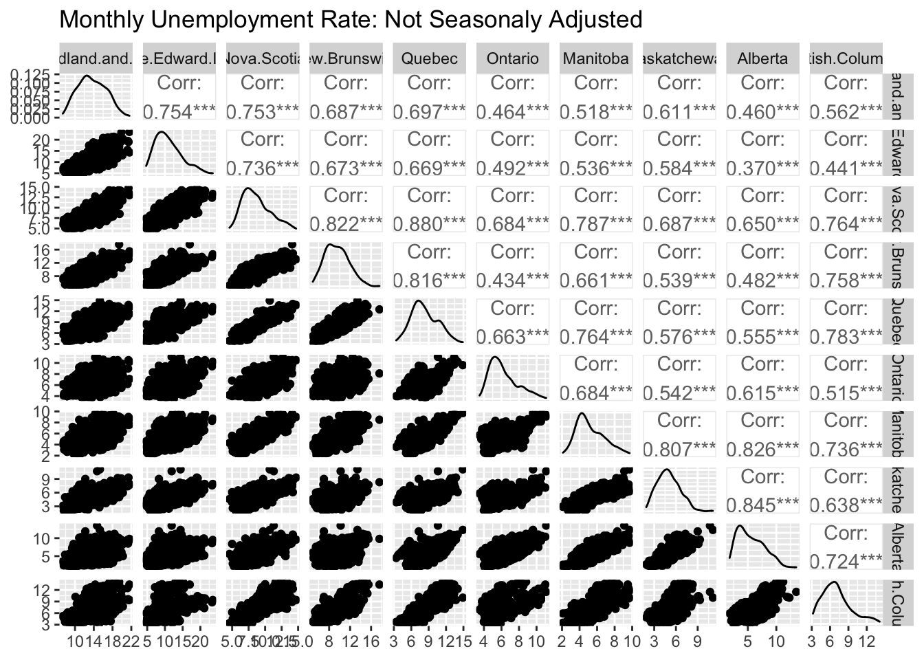

Plotting the Provinces as Time Series

We won’t bother pivoting the data table anymore, since it’s convenient for ggplot to have a column as an identifying feature.

Notice that the REF_DATE column is a character but it should be a date. We’ll use the lubridate package for converting into dates. The helpfile for the parse_date_time function is really useful for specifying the input format, as it clarifies that Y is a year with century but y is the two digit year without century. Using the wrong one will break the mutation.

data |> select(GEO,Sex,Age.group,Labour.force.characteristics,REF_DATE,VALUE,Data.type)|>
  filter(Sex == "Both sexes") |> 
  filter(GEO != "Canada")|> # since the Canada value will be a type of weighted average
  filter( Labour.force.characteristics == "Unemployment rate")|>
  filter(Age.group == "25 to 54 years")|>
  filter(Data.type == "Unadjusted")|>
  mutate(date = parse_date_time(REF_DATE, orders = "Y-m"))|> # convert from character date to date format.
  rename(unemployment.rate = VALUE)|>
  ggplot(aes(x=date, y = unemployment.rate, colour = GEO))+
  geom_line()+
  ggtitle("Unemployment Rates by Province")+
  theme(axis.text.x = element_text(angle = 90, vjust = 0.5, hjust=1))+# rotate axis labels so they don't overlap
  facet_wrap(~GEO)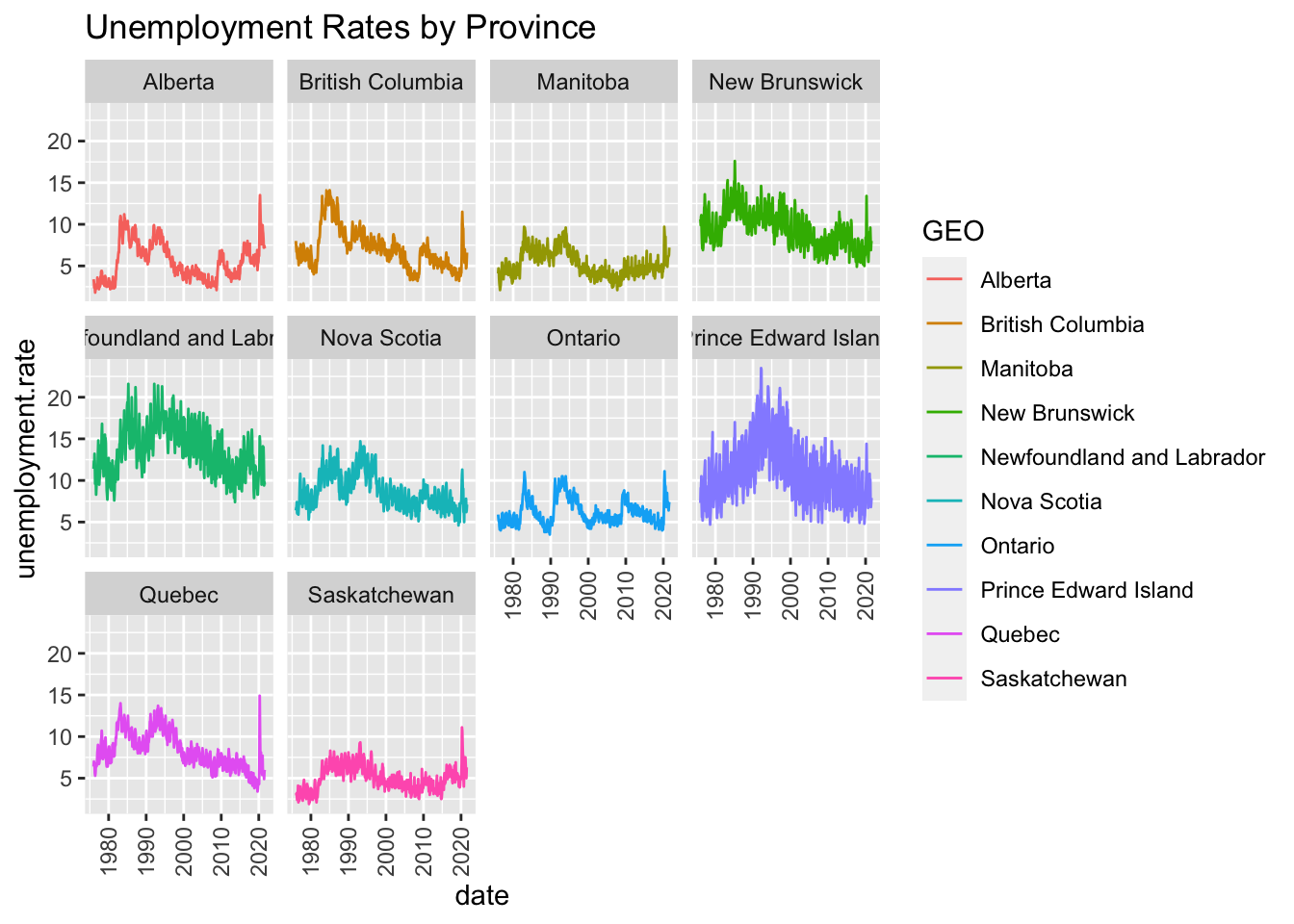

Plot the Within Year Seasonal Trends

Let’s split the date into year and month columns using the separate function. Then within a provincial facet we can plot each year as a different line. This figure makes lines darker as they go through the years by using year as the colour variable but highlights 2020-2021 in red using a second call to the geom_line function. There are a few strategies to do this, here I built a dataset with a new mutated variable specifying the 2020-2021 years and used it for plotting. This begins with a lot of filtering to obtain the ‘right’ data.

In some provinces, the strong seasonality of the unemployment rate realy pops out.

data4plot = data |> select(GEO,Sex,Age.group,Labour.force.characteristics,REF_DATE,VALUE,Data.type)|>
  filter(Sex == "Both sexes") |> 
  filter(GEO != "Canada")|> # since the Canada value will be a type of weighted average
  filter( Labour.force.characteristics == "Unemployment rate")|>
  filter(Age.group == "25 to 54 years")|>
  filter(Data.type == "Unadjusted")|>
  separate(REF_DATE, into = c("year","month"),sep = "-")|>#split year-month into year  month columns
  mutate(year = as.numeric(year))|>
  mutate(month = as.numeric(month))|>
  rename(unemployment.rate = VALUE)

  ggplot()+
  geom_line(data=data4plot,aes(x=month, y = unemployment.rate, colour = year, group = year))+
  # re-add in the pandemic year wwhile forcing the colour red
  geom_line(data=data4plot|> filter(year>2019),aes(x=month, y = unemployment.rate, group = year),colour = "red",lwd=1.24)+
    #add to the manual legend.
  scale_x_continuous(breaks = c(2,4,6,8,10))+
  ggtitle("Unadjusted Unemployment Rates by Province for 25 - 54 Year Olds: highlighting pandemic years")+
  facet_wrap(~GEO)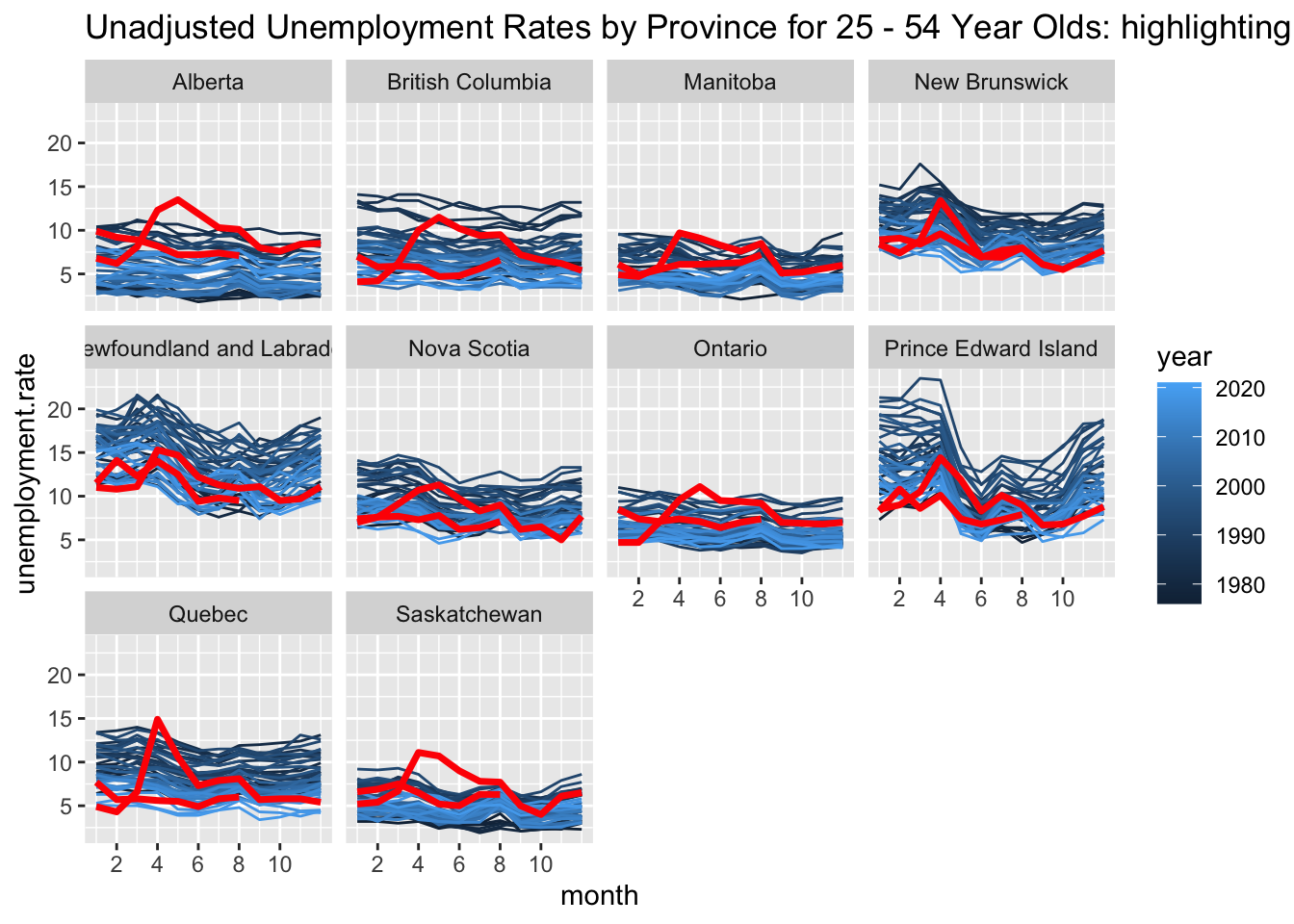

Plot the within year seasonal trends, but highlihght by decade

This figure uses a mutated variable defining the decade to set line colours, so 2020-2021 are inherrently already highlighted.

This time the Canadian average is included, despite the fact that it is a weighted average of the provincial values. Note that this time we are also keeping the filtered, mutated data to simplify merging datasets later.

unemployment = data |> select(GEO,Sex,Age.group,Labour.force.characteristics,REF_DATE,VALUE,Data.type)|>
  filter(Sex == "Both sexes") |> 
  # filter(GEO != "Canada")|> # since the Canada value will be a type of weighted average
  filter( Labour.force.characteristics == "Unemployment rate")|>
  filter(Age.group == "25 to 54 years")|>
  filter(Data.type == "Unadjusted")|>
  separate(REF_DATE, into = c("year","month"),sep = "-")|>#split year-month into year  month columns
  mutate(year = as.numeric(year))|>
  mutate(month = as.numeric(month))|>
  mutate(pandemic = 1+.1*as.numeric(as.numeric(year>=2020)))|>
  mutate(decade = factor(floor(year/10)*10 ))|>
  rename(unemployment.rate = VALUE)|>
  rename(province = GEO)
  


  ggplot(data = unemployment)+
  geom_line(aes(x=month, y = unemployment.rate, colour = decade, group = year))+
  scale_colour_brewer(palette = "Paired")+ # nicer colours
  scale_x_continuous(breaks = c(2,4,6,8,10))+ # place axis labels on even numbered months
  ggtitle("Unemployment Rates by Province")+
  facet_wrap(~province)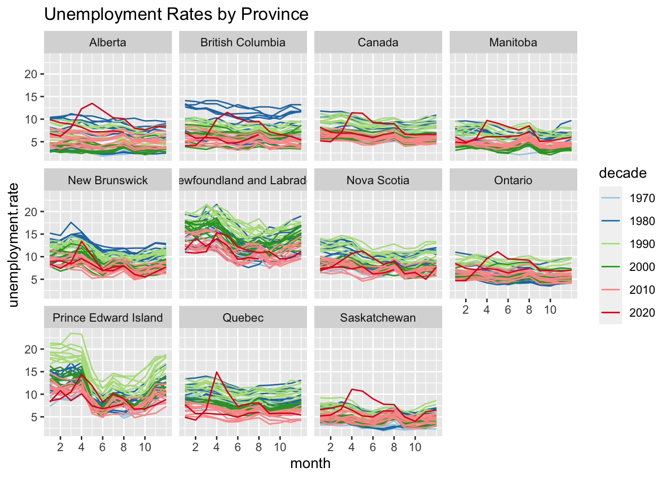

Housing starts

The housing starts are more complicated beacuse they are based on cities but the unemployment is based on provices

housing = get_cansim("34-10-0154-01") |> rename_all(make.names)

## Accessing CANSIM NDM product 34-10-0154 from Statistics Canada

## Parsing data

housing |> glimpse()

## Rows: 311,040
## Columns: 24
## $ REF_DATE                                  <chr> "1972-01", "1972-01", "1972-…
## $ GEO                                       <chr> "Census metropolitan areas",…
## $ DGUID                                     <chr> NA, NA, NA, NA, NA, NA, NA, …
## $ UOM                                       <chr> "Units", "Units", "Units", "…
## $ UOM_ID                                    <chr> "300", "300", "300", "300", …
## $ SCALAR_FACTOR                             <chr> "units", "units", "units", "…
## $ SCALAR_ID                                 <chr> "0", "0", "0", "0", "0", "0"…
## $ VECTOR                                    <chr> "v42127250", "v42127251", "v…
## $ COORDINATE                                <chr> "1.1.1", "1.1.2", "1.1.3", "…
## $ VALUE                                     <dbl> 7969, 3287, 615, 734, 3333, …
## $ STATUS                                    <chr> NA, NA, NA, NA, NA, NA, NA, …
## $ SYMBOL                                    <chr> NA, NA, NA, NA, NA, NA, NA, …
## $ TERMINATED                                <chr> NA, NA, NA, NA, NA, NA, NA, …
## $ DECIMALS                                  <chr> "0", "0", "0", "0", "0", "0"…
## $ GeoUID                                    <chr> NA, NA, NA, NA, NA, NA, NA, …
## $ Hierarchy.for.GEO                         <chr> "1", "1", "1", "1", "1", "1"…
## $ Classification.Code.for.Housing.estimates <chr> NA, NA, NA, NA, NA, NA, NA, …
## $ Hierarchy.for.Housing.estimates           <chr> "1", "1", "1", "1", "1", "2"…
## $ Classification.Code.for.Type.of.unit      <chr> NA, NA, NA, NA, NA, NA, NA, …
## $ Hierarchy.for.Type.of.unit                <chr> "1", "1.2", "1.3", "1.4", "1…
## $ val_norm                                  <dbl> 7969, 3287, 615, 734, 3333, …
## $ Date                                      <date> 1972-01-01, 1972-01-01, 197…
## $ Housing.estimates                         <fct> Housing starts, Housing star…
## $ Type.of.unit                              <fct> Total units, Single-detached…

# the unique cities
housing |> pull(GEO) |> unique()

##  [1] "Census metropolitan areas"                    
##  [2] "Brantford, Ontario"                           
##  [3] "Calgary, Alberta"                             
##  [4] "Edmonton, Alberta"                            
##  [5] "Greater Sudbury, Ontario"                     
##  [6] "Guelph, Ontario"                              
##  [7] "Halifax, Nova Scotia"                         
##  [8] "Hamilton, Ontario"                            
##  [9] "Kingston, Ontario"                            
## [10] "Kitchener-Cambridge-Waterloo, Ontario"        
## [11] "London, Ontario"                              
## [12] "Moncton, New Brunswick"                       
## [13] "Montréal excluding Saint-Jérôme, Quebec"      
## [14] "Ottawa-Gatineau, Ontario/Quebec"              
## [15] "Ottawa-Gatineau, Ontario part, Ontario/Quebec"
## [16] "Ottawa-Gatineau, Quebec part, Ontario/Quebec" 
## [17] "Peterborough, Ontario"                        
## [18] "Québec, Quebec"                               
## [19] "Regina, Saskatchewan"                         
## [20] "St. Catharines-Niagara, Ontario"              
## [21] "St. John's, Newfoundland and Labrador"        
## [22] "Saint John, New Brunswick"                    
## [23] "Saguenay, Quebec"                             
## [24] "Saskatoon, Saskatchewan"                      
## [25] "Thunder Bay, Ontario"                         
## [26] "Toronto, Ontario"                             
## [27] "Vancouver, British Columbia"                  
## [28] "Victoria, British Columbia"                   
## [29] "Windsor, Ontario"                             
## [30] "Winnipeg, Manitoba"                           
## [31] "Kelowna, British Columbia"                    
## [32] "Oshawa, Ontario"                              
## [33] "Barrie, Ontario"                              
## [34] "Trois-Rivières, Quebec"                       
## [35] "Abbotsford-Mission, British Columbia"         
## [36] "Sherbrooke, Quebec"                           
## [37] "Montréal, Quebec"

To merge the housing starts with the unemployment, we need to set both to the same measurement unit, provinces per {month, year}. To construct provincial housing starts, sum over the municipailites within a province. Many of these StatCan tables have multiple data types, so we will only consider Housing.estimates = “Housing starts” and Type.of.unit = “Total units”.

Notice that Ottawa-Gatineau is split into ON and QC parts.

Let’s use the separate function to split apart the province and city. Considering the GEO location “Ottawa-Gatineau, Ontario part, Ontario/Quebec” and splitting at the “,” we can end up with some innaccurate provinces “Ontario/Quebec” or destroy the useful location information by removing “Ontario part”.

Here are a few options using regular expressions. Note that most of these give warnings, generally complaining about the GEO location “Census metropolitan areas”. Strategies to split the GEO location at commas will result in NA’s since this location has no comma. Those warnings are left in the output below.

# set up city by replacing everything after the first "," with "":
housing |> mutate(city = str_replace_all(GEO, pattern = "(,\\s).*", replacement ="")) |> 
  pull(city) |> unique() |> head(16)

##  [1] "Census metropolitan areas"       "Brantford"                      
##  [3] "Calgary"                         "Edmonton"                       
##  [5] "Greater Sudbury"                 "Guelph"                         
##  [7] "Halifax"                         "Hamilton"                       
##  [9] "Kingston"                        "Kitchener-Cambridge-Waterloo"   
## [11] "London"                          "Moncton"                        
## [13] "Montréal excluding Saint-Jérôme" "Ottawa-Gatineau"                
## [15] "Peterborough"                    "Québec"

#Split everything at the last comma:
# Separate GEO at a ", ", but if more than one exists find the one which is NOT followed by any characters, then a comma:
#Notice how this handles the Ontario and Quebec parts of the Ottawa-Gatineau region
housing |> separate(GEO, into  = c("city","province"), sep = ",\\s(?!(.*,))") |> 
  select(city,  province) |>
  unique()|> head(16)

## Warning: Expected 2 pieces. Missing pieces filled with `NA` in 8940 rows [1, 2,
## 3, 4, 5, 6, 7, 8, 9, 10, 11, 12, 13, 14, 15, 451, 452, 453, 454, 455, ...].

## # A tibble: 16 × 2
##    city                            province      
##    <chr>                           <chr>         
##  1 Census metropolitan areas       <NA>          
##  2 Brantford                       Ontario       
##  3 Calgary                         Alberta       
##  4 Edmonton                        Alberta       
##  5 Greater Sudbury                 Ontario       
##  6 Guelph                          Ontario       
##  7 Halifax                         Nova Scotia   
##  8 Hamilton                        Ontario       
##  9 Kingston                        Ontario       
## 10 Kitchener-Cambridge-Waterloo    Ontario       
## 11 London                          Ontario       
## 12 Moncton                         New Brunswick 
## 13 Montréal excluding Saint-Jérôme Quebec        
## 14 Ottawa-Gatineau                 Ontario/Quebec
## 15 Ottawa-Gatineau, Ontario part   Ontario/Quebec
## 16 Ottawa-Gatineau, Quebec part    Ontario/Quebec

#Build the province by splitting at the first comma, then adjusting the province by 
# handing cases such as "Ontario part, Ontario/Quebec"
# notice that I'm actually splitting at all commas and allowing anything after the 
# second comma (where it exists) to be discarded.
housing |> separate(GEO, into  = c("city","province"), sep = ",\\s") |> 
  mutate(province = str_replace_all(province, pattern = " part", replacement = ""))|>
  select(city,  province)|> unique()|> head(16)

## Warning: Expected 2 pieces. Additional pieces discarded in 17880 rows [211, 212,
## 213, 214, 215, 216, 217, 218, 219, 220, 221, 222, 223, 224, 225, 226, 227, 228,
## 229, 230, ...].

## Warning: Expected 2 pieces. Missing pieces filled with `NA` in 8940 rows [1, 2,
## 3, 4, 5, 6, 7, 8, 9, 10, 11, 12, 13, 14, 15, 451, 452, 453, 454, 455, ...].

## # A tibble: 16 × 2
##    city                            province      
##    <chr>                           <chr>         
##  1 Census metropolitan areas       <NA>          
##  2 Brantford                       Ontario       
##  3 Calgary                         Alberta       
##  4 Edmonton                        Alberta       
##  5 Greater Sudbury                 Ontario       
##  6 Guelph                          Ontario       
##  7 Halifax                         Nova Scotia   
##  8 Hamilton                        Ontario       
##  9 Kingston                        Ontario       
## 10 Kitchener-Cambridge-Waterloo    Ontario       
## 11 London                          Ontario       
## 12 Moncton                         New Brunswick 
## 13 Montréal excluding Saint-Jérôme Quebec        
## 14 Ottawa-Gatineau                 Ontario/Quebec
## 15 Ottawa-Gatineau                 Ontario       
## 16 Ottawa-Gatineau                 Quebec

#note that this leaves in an artifact province :"Ontario/Quebec" from Ottawa-Gatineau 
# but that is a combo of the Ontario part and the Quebec part
# that province combo could be replaced with NA and then eliminated later
# for example:

housing |> separate(GEO, into  = c("city","province"), sep = ",\\s") |> 
  mutate(province = str_replace_all(province, pattern = " part", replacement = ""))|>
  mutate(province = str_replace_all(province, pattern = "Ontario/Quebec", replacement = "NA"))|>
  select(city,  province)|> unique()|> head(16)

## Warning: Expected 2 pieces. Additional pieces discarded in 17880 rows [211, 212,
## 213, 214, 215, 216, 217, 218, 219, 220, 221, 222, 223, 224, 225, 226, 227, 228,
## 229, 230, ...].

## Warning: Expected 2 pieces. Missing pieces filled with `NA` in 8940 rows [1, 2,
## 3, 4, 5, 6, 7, 8, 9, 10, 11, 12, 13, 14, 15, 451, 452, 453, 454, 455, ...].

## # A tibble: 16 × 2
##    city                            province     
##    <chr>                           <chr>        
##  1 Census metropolitan areas       <NA>         
##  2 Brantford                       Ontario      
##  3 Calgary                         Alberta      
##  4 Edmonton                        Alberta      
##  5 Greater Sudbury                 Ontario      
##  6 Guelph                          Ontario      
##  7 Halifax                         Nova Scotia  
##  8 Hamilton                        Ontario      
##  9 Kingston                        Ontario      
## 10 Kitchener-Cambridge-Waterloo    Ontario      
## 11 London                          Ontario      
## 12 Moncton                         New Brunswick
## 13 Montréal excluding Saint-Jérôme Quebec       
## 14 Ottawa-Gatineau                 NA           
## 15 Ottawa-Gatineau                 Ontario      
## 16 Ottawa-Gatineau                 Quebec

Preparing for Merging Datasets

Here we rebuild the dataset and sum housing starts within provinces to obtain

# We will keep the final strategy above, but also mutate in the
# Housing.estimates  and Type.of.unit
# select fewer variables, to clean it up prior to merging datasets
housing.starts = housing |> separate(GEO, into  = c("city","province"), sep = ",\\s") |> 
  mutate(province = str_replace_all(province, pattern = " part", replacement = ""))|>
  mutate(province = str_replace_all(province, pattern = "Ontario/Quebec", replacement = "NA"))|>
  rename(housing.starts = VALUE)|> # so I'm not confused later
  filter(Housing.estimates == "Housing starts")|>
  filter(Type.of.unit == "Total units") |>
  filter(!is.na(province))|> # get rid of census metropolitan areas
  mutate(date = parse_date_time(REF_DATE, orders = "Y-m"))|> # convert from character date to date format.
  separate(REF_DATE, into = c("year","month"),sep = "-")|>#split year-month into year  month columns
  mutate(year = as.numeric(year))|>
  mutate(month = as.numeric(month))|>
  group_by(province, year, month, date) |> # look within provinces at a given time
  summarize(total.housing = sum(housing.starts)) |>
  ungroup()

## Warning: Expected 2 pieces. Additional pieces discarded in 17880 rows [211, 212,
## 213, 214, 215, 216, 217, 218, 219, 220, 221, 222, 223, 224, 225, 226, 227, 228,
## 229, 230, ...].

## Warning: Expected 2 pieces. Missing pieces filled with `NA` in 8940 rows [1, 2,
## 3, 4, 5, 6, 7, 8, 9, 10, 11, 12, 13, 14, 15, 451, 452, 453, 454, 455, ...].

## `summarise()` has grouped output by 'province', 'year', 'month'. You can override using the `.groups` argument.

housing.starts |> glimpse()

## Rows: 5,960
## Columns: 5
## $ province      <chr> "Alberta", "Alberta", "Alberta", "Alberta", "Alberta", "…
## $ year          <dbl> 1972, 1972, 1972, 1972, 1972, 1972, 1972, 1972, 1972, 19…
## $ month         <dbl> 1, 2, 3, 4, 5, 6, 7, 8, 9, 10, 11, 12, 1, 2, 3, 4, 5, 6,…
## $ date          <dttm> 1972-01-01, 1972-02-01, 1972-03-01, 1972-04-01, 1972-05…
## $ total.housing <dbl> 597, 1104, 1372, 1639, 2324, 2414, 1335, 1481, 1260, 103…

Clean up extraneous columns, and merge datasets:

By default inner_join will merge two datasets based on their common column names. Only rows which appear in both datasets will be kept.

both =  unemployment |>
  select(province, year, month, decade,pandemic, unemployment.rate) |> 
  inner_join(housing.starts)

## Joining, by = c("province", "year", "month")

both |> glimpse()

## Rows: 4,932
## Columns: 8
## $ province          <chr> "Newfoundland and Labrador", "Nova Scotia", "New Bru…
## $ year              <dbl> 1976, 1976, 1976, 1976, 1976, 1976, 1976, 1976, 1976…
## $ month             <dbl> 1, 1, 1, 1, 1, 1, 1, 1, 1, 2, 2, 2, 2, 2, 2, 2, 2, 2…
## $ decade            <fct> 1970, 1970, 1970, 1970, 1970, 1970, 1970, 1970, 1970…
## $ pandemic          <dbl> 1, 1, 1, 1, 1, 1, 1, 1, 1, 1, 1, 1, 1, 1, 1, 1, 1, 1…
## $ unemployment.rate <dbl> 11.4, 6.4, 10.6, 6.4, 5.9, 4.1, 3.2, 3.4, 8.0, 12.3,…
## $ date              <dttm> 1976-01-01, 1976-01-01, 1976-01-01, 1976-01-01, 197…
## $ total.housing     <dbl> 40, 273, 99, 3638, 3264, 333, 219, 1239, 1416, 51, 6…

Comparing Unemployment and Housing Starts

Note that there are Prince Edward Island and the territories not represented within the housing starts dataset and therefore are not in the following plots.

In general as unemployment increases, housing starts decrease.

both |> ggplot(aes(x=unemployment.rate, y =total.housing))+
  geom_point( aes(colour =  province, group = province),alpha = .1)+#alpha is the transparancy of the points
  ggpubr::stat_regline_equation()+
  geom_smooth(method = "lm")+
  facet_wrap(~province)

## `geom_smooth()` using formula 'y ~ x'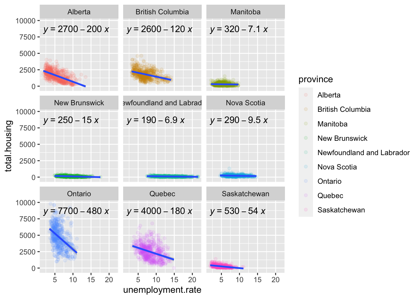

Going Further

Make residual plots for the linear regessions
Consider other variables/ relationship, such as CPI from table 18-10-0004-01 Consumer Price Index, monthly, not seasonally adjusted
Consider looking for a time varying trend, subsetting the years, or even multiple regression with a year effect.

Cansim Library for Socio-Economic data