Possible analysis and Keywords
- Time Series
- Spatial Data Set
- Stacked Area Chart
- School Revenue
- Education Data
Data Provider
The provincial government of Ontaio provides open access to thousands of data sets via their Open Data Ontario portal. The purpose of sharing all data documents with the public is to remain transparent and accessible. More details about the data license, training materials, and other information can be found here.
Private Elementary and Secondary Schools Revenues, by Direct Source of Funds
This dataset contains 138 observations across provinces and funding sources from 1947 to 2002.
The dataset and its metadata file which contains detailed variable descriptions have been stored together as a zip file. The data resource and its description can be found here, you also can quickly discover the customized table here.
Exploratory Analysis
Organizing Dataset
The following code is used to download and organize the original dataset, and only select the important variables to form a new dataset.
# library
library(tidyverse)
library(viridis)
library(hrbrthemes)

# Download the zip file of school revenues dataset
temp <- tempfile()
download.file("https://www150.statcan.gc.ca/n1/tbl/csv/37100084-eng.zip",temp)
(file_list <- as.character(unzip(temp, list = TRUE)$Name))
## [1] "37100084.csv" "37100084_MetaData.csv"revenue <- read_csv(unz(temp, "37100084.csv"))
unlink(temp) # Delete temp file
# Organize the dataset
revenue <- revenue |>
separate(REF_DATE, c("year", "year.end"), "/") |>
mutate(year = as.numeric(year))|>
drop_na(VALUE) |>
rename_all(make.names)
# take a look at the data:
revenue |> glimpse()## Rows: 4,163
## Columns: 16
## $ year <dbl> 1947, 1947, 1947, 1947, 1947, 1947, 1947, 1947,…
## $ year.end <chr> "1948", "1948", "1948", "1948", "1948", "1948",…
## $ GEO <chr> "Canada", "Canada", "Canada", "Canada", "Canada…
## $ DGUID <lgl> NA, NA, NA, NA, NA, NA, NA, NA, NA, NA, NA, NA,…
## $ Direct.source.of.funds <chr> "Total revenues", "Government sources", "Federa…
## $ UOM <chr> "Dollars", "Dollars", "Dollars", "Dollars", "Do…
## $ UOM_ID <dbl> 81, 81, 81, 81, 81, 81, 81, 81, 81, 81, 81, 81,…
## $ SCALAR_FACTOR <chr> "thousands", "thousands", "thousands", "thousan…
## $ SCALAR_ID <dbl> 3, 3, 3, 3, 3, 3, 3, 3, 3, 3, 3, 3, 3, 3, 3, 3,…
## $ VECTOR <chr> "v1444638", "v1444642", "v1444639", "v1444640",…
## $ COORDINATE <dbl> 1.1, 1.5, 1.2, 1.3, 1.4, 1.8, 1.9, 1.1, 6.1, 6.…
## $ VALUE <dbl> 13951, 0, 0, 0, 0, 4114, 0, 9837, 743, 0, 0, 0,…
## $ STATUS <chr> NA, NA, NA, NA, NA, NA, NA, NA, NA, NA, NA, NA,…
## $ SYMBOL <lgl> NA, NA, NA, NA, NA, NA, NA, NA, NA, NA, NA, NA,…
## $ TERMINATED <lgl> NA, NA, NA, NA, NA, NA, NA, NA, NA, NA, NA, NA,…
## $ DECIMALS <dbl> 0, 0, 0, 0, 0, 0, 0, 0, 0, 0, 0, 0, 0, 0, 0, 0,…School Revenue by Different Funded Source in Canada
The following code is used to draw the stacked area chart so that we can directly see the time-series trend and proportion of different funding sources over the years.
# Subset a reveune dataset which only focus on different funding source in Canada and plot the graph
revenue |> subset( GEO == "Canada" & Direct.source.of.funds != "Total revenues")|>
ggplot( aes(x=year, y=VALUE, group=Direct.source.of.funds, colour =Direct.source.of.funds)) +
    geom_line(alpha=0.6 , size=.5) +
    scale_fill_viridis(discrete = T) +
    theme_ipsum() +
    labs(title = "School Revenue Funded \n from Different Sources")+
  theme(axis.text.x = element_text(angle = 90, vjust = 0.5, hjust=1))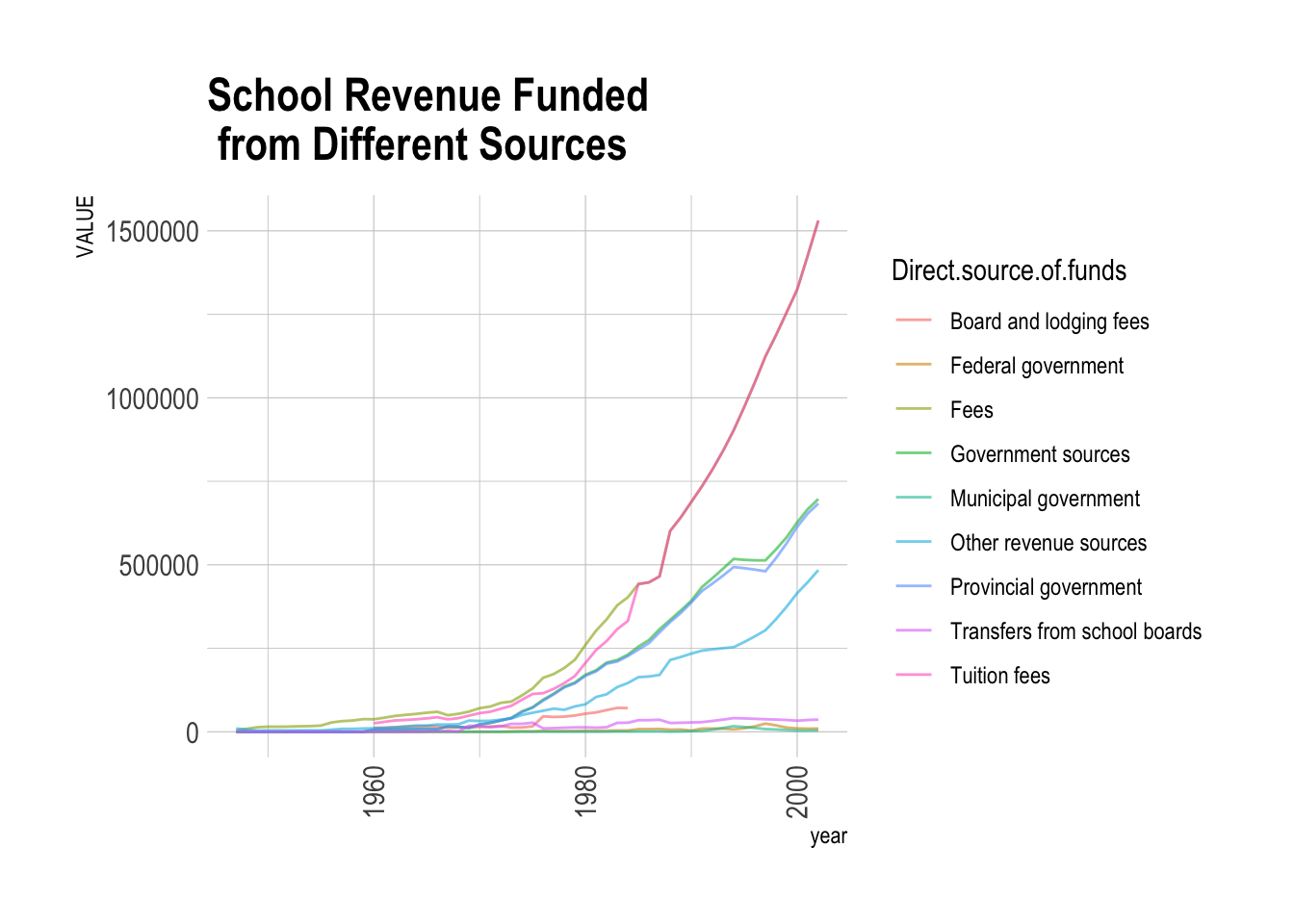
Total School Revenue in Different Provinces
The following code is used to draw the stacked area chart so that we can directly see the time-series trend and proportion in different provinces over the years.
# Subset a reveune dataset which only focuses on different funding source in Canada and plot the graph
revenue |> subset( GEO != "Canada" & Direct.source.of.funds == "Total revenues")|>
ggplot( aes(x=year, y=VALUE, group=GEO, colour =GEO)) +
    geom_line(alpha=0.6 , size=.5) +
    scale_fill_viridis(discrete = T) +
    theme_ipsum() +
    ggtitle("Total School Revenue Funded \n in Different Provinces")+
  theme(axis.text.x = element_text(angle = 90, vjust = 0.5, hjust=1))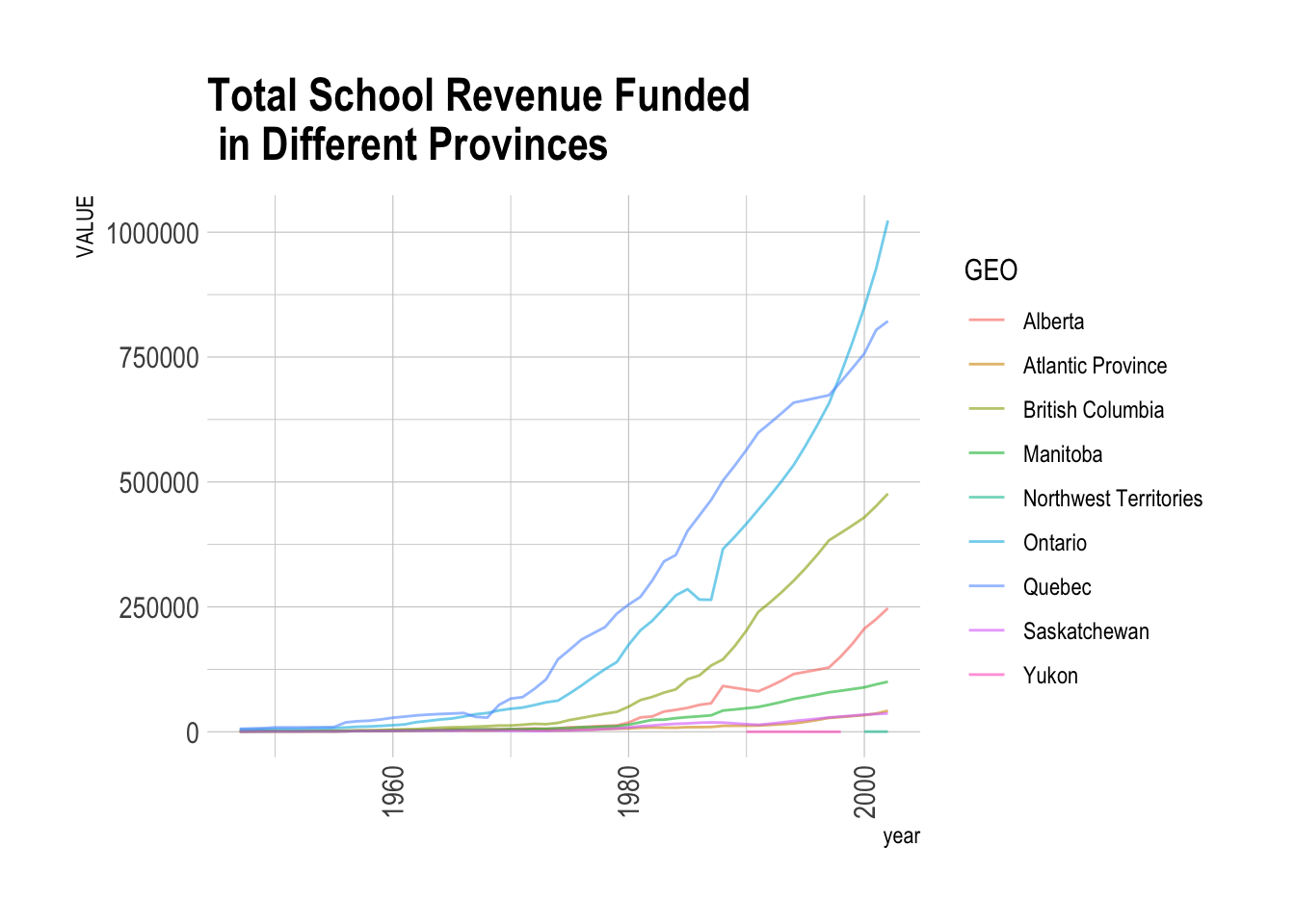
Tidy the variables
There are quite a few variables that aren’t really of interest like SCALAR_ID and COORDINATE, while other variables are hidden within the single column Direct.source.of.funds. Here we wish to rearrange the data from a tall format into a wider format. The function pivot_wider takes a column and spreads its factors into new columns. This makes the observational unit combinations of year and GEO.
# select the columns of interest
revenue_wide = revenue |>
      select(year, GEO, Direct.source.of.funds, VALUE) |>
  # pivot wider by taking factors from Direct.source.of.funds
  # fill in the variable with values from VALUE
      pivot_wider(names_from = Direct.source.of.funds, values_from = VALUE) |>
  # rebuild the variable names so that they do not have spaces
      rename_all(make.names)

revenue_wide |> glimpse()
## Rows: 452
## Columns: 12
## $ year <dbl> 1947, 1947, 1947, 1947, 1947, 1947, 1947,…
## $ GEO <chr> "Canada", "Atlantic Province", "Quebec", …
## $ Total.revenues <dbl> 13951, 743, 5900, 4509, 556, 449, 529, 12…
## $ Government.sources <dbl> 0, 0, 0, 0, 0, 0, 0, 0, NA, 0, 0, 0, 0, 0…
## $ Federal.government <dbl> 0, 0, 0, 0, 0, 0, 0, 0, NA, 0, 0, 0, 0, 0…
## $ Provincial.government <dbl> 0, 0, 0, 0, 0, 0, 0, 0, NA, 0, 0, 0, 0, 0…
## $ Municipal.government <dbl> 0, 0, 0, 0, 0, 0, 0, 0, NA, 0, 0, 0, 0, 0…
## $ Fees <dbl> 4114, 144, 1770, 1377, 299, 59, 87, 378, …
## $ Transfers.from.school.boards <dbl> 0, 0, 0, 0, 0, 0, 0, 0, NA, 0, 0, 0, 0, 0…
## $ Other.revenue.sources <dbl> 9837, 599, 4130, 3132, 257, 390, 442, 887…
## $ Tuition.fees <dbl> NA, NA, NA, NA, NA, NA, NA, NA, NA, NA, N…
## $ Board.and.lodging.fees <dbl> NA, NA, NA, NA, NA, NA, NA, NA, NA, NA, N…Wider data makes easier plotting and analysis
To predict the school fees, one would need to consider the other sources of funding. Such a regression model can’t be directly made without first widening the data. Below, the variables are plotted against each other and a basic linear model is performed.
library(GGally)
revenue_wide |>
  filter(GEO=="Canada") |>
 ggpairs()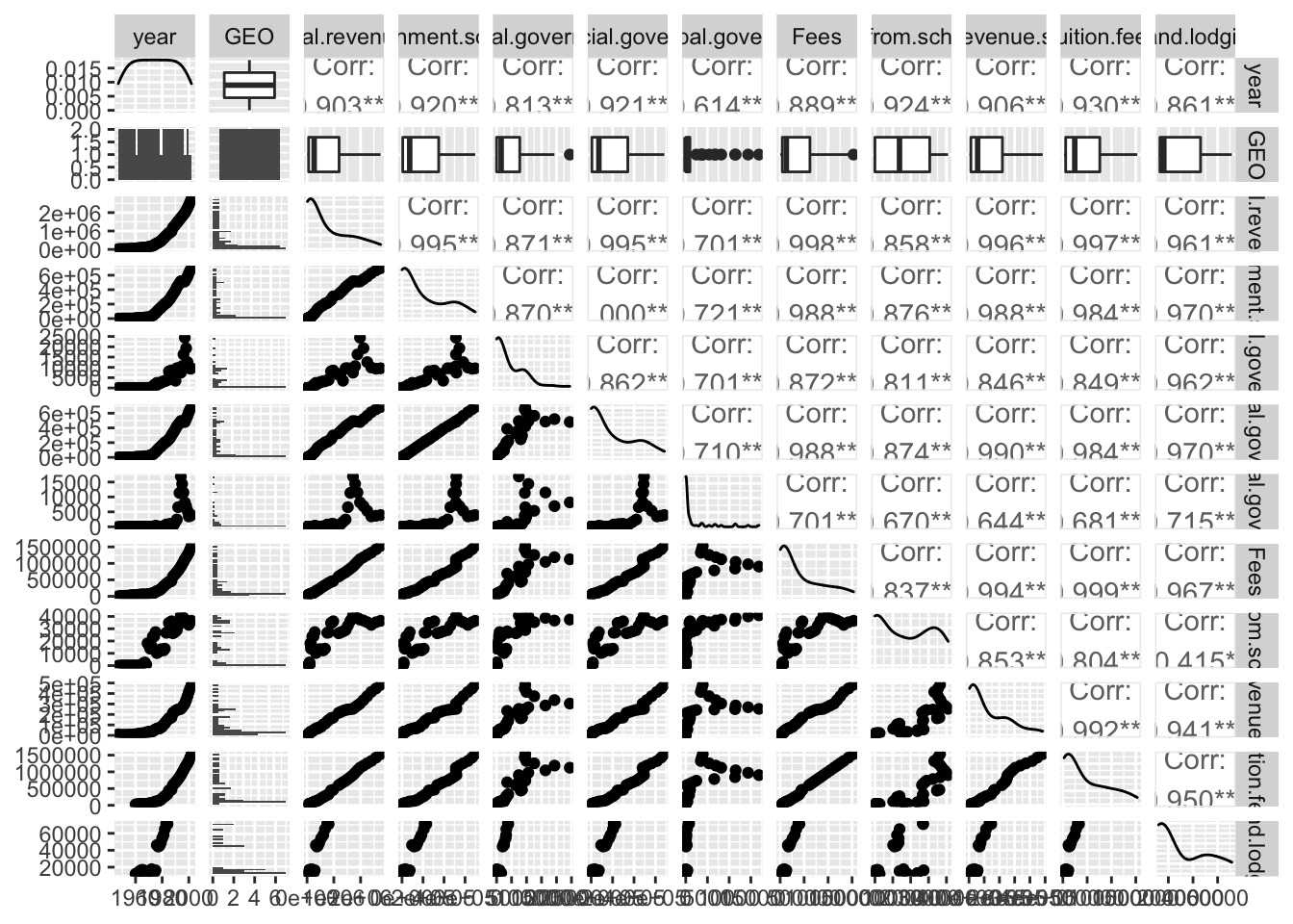
CanadaWide = revenue_wide |>
  filter(GEO=="Canada")
lm(Fees~Transfers.from.school.boards+Municipal.government+Provincial.government+Federal.government,CanadaWide)
##
## Call:
## lm(formula = Fees ~ Transfers.from.school.boards + Municipal.government +
## Provincial.government + Federal.government, data = CanadaWide)
##
## Coefficients:
## (Intercept) Transfers.from.school.boards
## 17835.680 -4.073
## Municipal.government Provincial.government
## -0.783 2.094
## Federal.government
## 8.957