Possible Analysis and Keywords
- Linear Chart
- Time Series
- Data Merging and Cleaning
- Soft Drinks
- Manufacturing Data ## Data Provider
Statistics Canada’s Open Government is a free and open-access platform containing over 80,000 datasets across diverse subjects. The purpose of sharing all data documents with the public is to remain transparent and accessible.
Dataset can be discovered by multiple searching methods here, such as Browse by subject, Open Government Portal for direct keywords search, Open Maps which contains geospatial information data, Open Data Inventory from the government of Canada organization, Apps Gallery for representing those mobile and web-based application data, Open Data 101 for letting people know how to use dataset and so on.
Food Manufacturing: Annual Soft Drink Production
A dataset recording the soft drink production every quarter from 1950 to 1977, its supporting documentation can be found here, you also can quickly discover the customized table here.
The dataset switched to monthly soft drinks production from 1976 to 1995. Its supporting documentation can be found here, you also can quickly discover the customized table here.
All datasets and their metadata files including detailed variable descriptions are stored as a zip file. The variables in the data sets are dates and production variables recorded in units of thousands of gallons on a monthly, quarterly, and annual basis.
Exprolary Analysis
Data loading
The following code is used to organize monthly and annual orginal datasets, and merge them into one quarterly soft drink production dataset from 1950 to 1995.
# library
library(tidyverse)
library(lubridate)

#Download the zip file of QUARTERLY soft drink production AND rearrange the dataset
temp <- tempfile()
download.file("https://www150.statcan.gc.ca/n1/tbl/csv/16100100-eng.zip",temp)
(file_list <- as.character(unzip(temp, list = TRUE)$Name))
## [1] "16100100.csv" "16100100_MetaData.csv"quarterlydata <- read_csv(unz(temp, "16100100.csv"))
unlink(temp) # Delete temp file
# Organize the quarterly dataset
quarterly = quarterlydata |> mutate(REF_DATE = as_date(paste(REF_DATE,"-1",sep ="")))
quarterly = quarterly |> rename(quarter = REF_DATE, QuarterlyValue = VALUE)|>
select(quarter, QuarterlyValue)
#Download the zip file of MONTHLY soft drink production AND rearrange the dataset
temp <- tempfile()
download.file("https://www150.statcan.gc.ca/n1/tbl/csv/16100099-eng.zip",temp)
(file_list <- as.character(unzip(temp, list = TRUE)$Name))## [1] "16100099.csv" "16100099_MetaData.csv"monthlydata <- read_csv(unz(temp, "16100099.csv"))
unlink(temp)
monthlydata = monthlydata |> rename(date = REF_DATE, Produced = VALUE)
# It is necessary to add the month and day values at the end of the year data before running as.Date() function. Since the original CSV file has its default data format, we need to fill out the missing parts of the date, which is date data in this case, as the character format, then use the as.Date() function to convert.
monthly <- monthlydata |>
mutate(date = as_date(paste(date,"-1",sep ="")))|>
select(date, Produced)
# Now we want to extend the quarterly data set by combining over the monthly dataset:
MoreQuarters <- monthly |>
mutate(quarter = quarter(date,with_year = TRUE)) |>
group_by(quarter) |>
mutate(QuarterlyValue = sum(Produced))|>
select(date, quarter, QuarterlyValue) |>
distinct( quarter, QuarterlyValue, .keep_all=TRUE) |>
ungroup() |>
select(date, QuarterlyValue) |>
rename(quarter = date)
AllQuarters = rbind(quarterly,MoreQuarters)
# Create the dataset of annual soft drink production by summarizing the quaterly production value by year
annual = AllQuarters |>
mutate(Year = floor_date(AllQuarters$quarter, unit = "year")) |>
group_by(Year) |>
mutate(AnnualValue = sum(QuarterlyValue))|>
select(Year, AnnualValue) |>
distinct( Year, AnnualValue)
head(AllQuarters)## # A tibble: 6 × 2
## quarter QuarterlyValue
## <date> <dbl>
## 1 1950-01-01 19349
## 2 1950-04-01 29730
## 3 1950-07-01 31721
## 4 1950-10-01 20045
## 5 1951-01-01 17398
## 6 1951-04-01 25893head(annual)## # A tibble: 6 × 2
## # Groups: Year [6]
## Year AnnualValue
## <date> <dbl>
## 1 1950-01-01 100845
## 2 1951-01-01 91691
## 3 1952-01-01 101396
## 4 1953-01-01 107892
## 5 1954-01-01 103816
## 6 1955-01-01 116301head(monthly)## # A tibble: 6 × 2
## date Produced
## <date> <dbl>
## 1 1976-01-01 20680
## 2 1976-02-01 23392
## 3 1976-03-01 21553
## 4 1976-04-01 24304
## 5 1976-05-01 27791
## 6 1976-06-01 32838Soft drink production
### Plot the graph of annual and quaterly soft drink production
ggplot(annual, aes(x = Year, y = AnnualValue, group = 1)) +
  geom_line() +
  ggtitle("Annual soft drink production")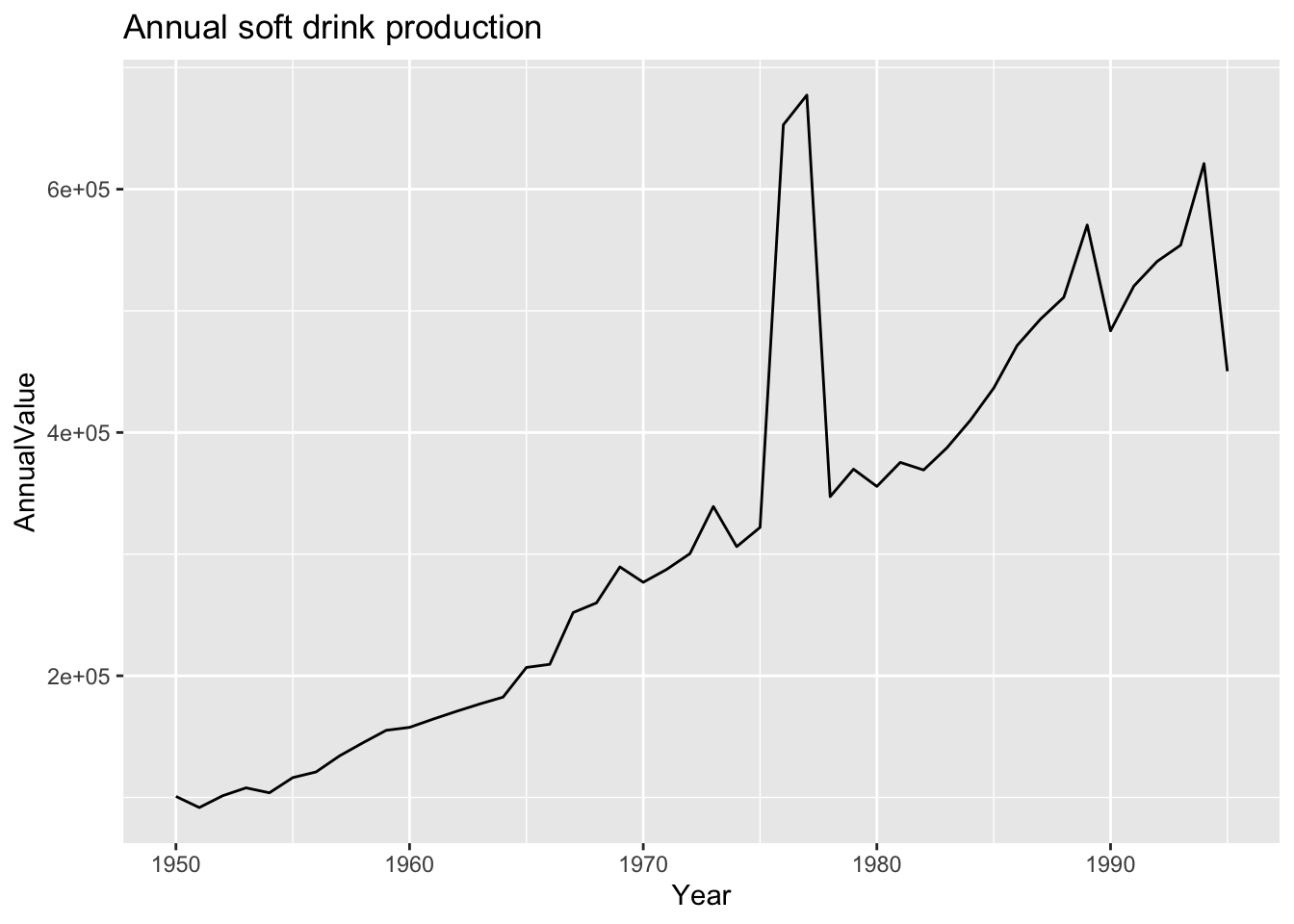
ggplot(AllQuarters, aes(x = quarter, y = QuarterlyValue, group = 1)) +
  geom_line() +
  geom_point(position="jitter") +
  ggtitle("Quaterly soft drink production")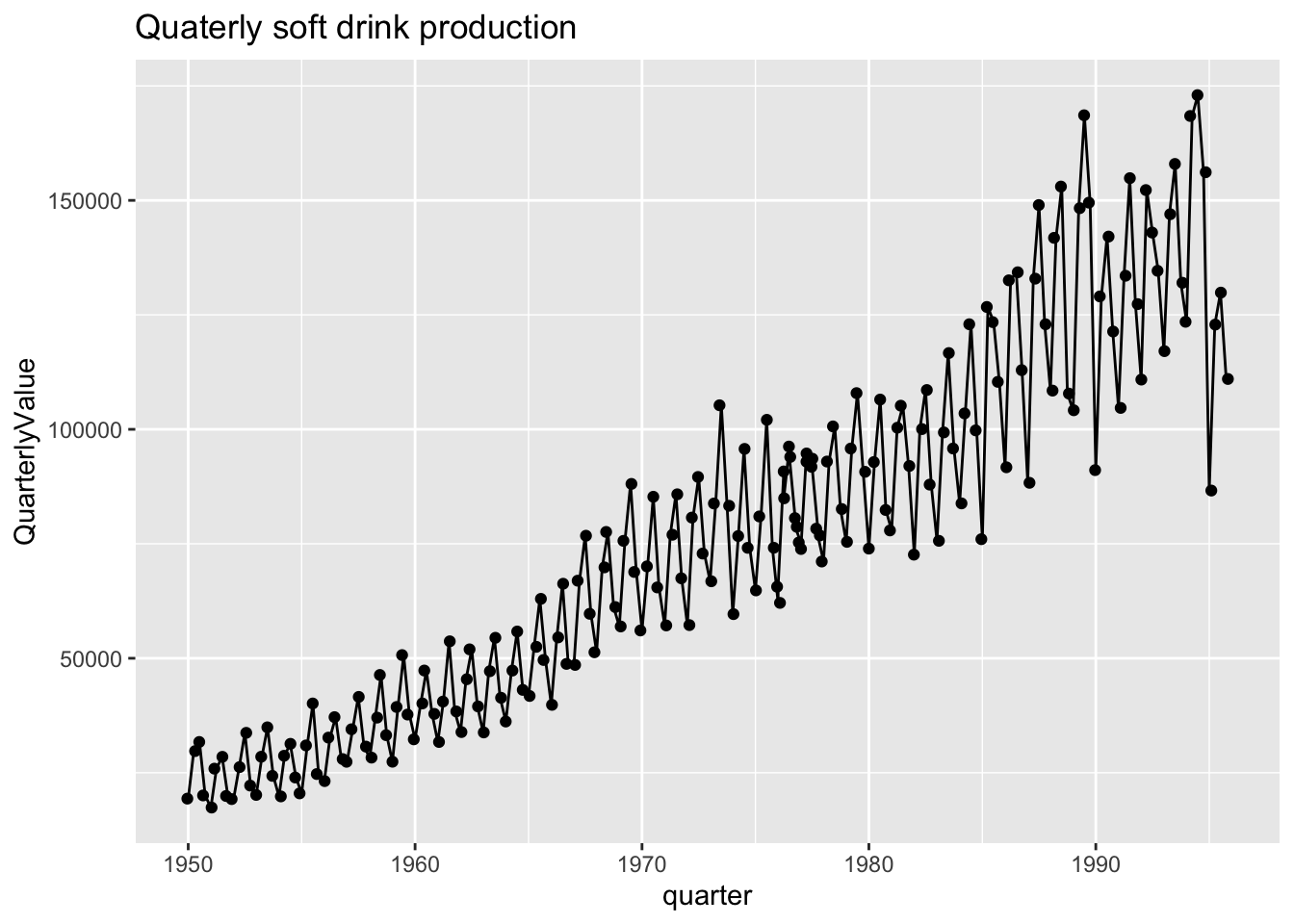
ggplot(monthly, aes(x = date, y = Produced, group = 1)) +
  geom_line() +
  ggtitle("Monthly soft drink production")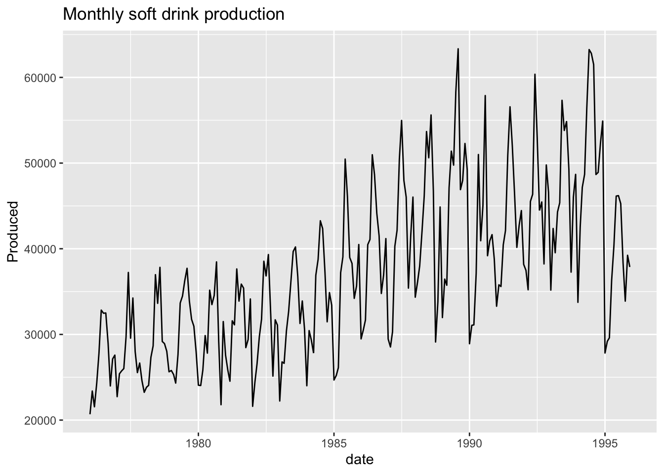
- What happened to the annual data from 1976 and 1977? Need a hint, Zoomm in by changing the x axis limits by adding this to the ggplot:
#xlim(as_date(c("1970-01-01","1980-12-01")))- Need another hint? Look back at the quarterly data sets before they were combined from different sources.
Quarterly soft drink production, just the old dataset
To better see the production proportions across the four quarters in each year, the following code is used to plot the stacked percentage bar plots of quarterly soft drink production.
- Check out how the Year-Month-Date is split into its elements using separate:
# Use separate() function form tidyr package to take the date variable apart into year and month

 quarterly |>
  separate( quarter, into = c("year","month", "date"), sep = "-") |>
# Stacked + percent
ggplot( aes(fill=month, y= QuarterlyValue, x=as.Date(year,"%Y"))) +
  geom_bar(position="fill", stat="identity") +
  ggtitle("Percent Stacked Barchart of Quaterly Soft Drink Production") +
  xlab("Year") +
  ylab("Percentage")+
  theme(axis.text.x = element_text(angle = 90, vjust = 0.5, hjust=1))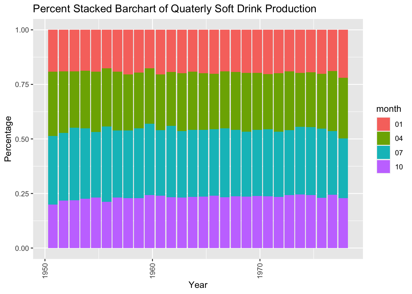
Summary
- The percent produced in each quarter is reasonably stable.