Possible Analysis and Keywords

Linear Regression
Time Series
Spatial Data Set
Bar Plot
Official Language
Median Income
Population
Census Data

Data Provider

Census Mapper provides an API for accessing Statistics Canada census data. Censusmapper is provided by Jens von Bergman who is a regular in the news for publishing civic data and maps. Find him also on his Twitter account. All data are taken from Statistics Canada and governed by Statistics Canada Open Data Licence.

You can use the Census Mapper website, but it is easier (to reproduce and modify) if we use the associated cancensus R package. Click that link for an excellent vignette including how to sign up for an API key to obtain your own data. Note that there are quota limits for an API key. More details on API sign up and usage below.

CensusMapper

The easiest way to get exact data information from CensusMapper is to pick specific census year and variables, and regions.

The available year selections related to census data are from 2001, 2006, 2011, and 2016, also the year selection among tax data are available is from 2000 to 2017.
The region selection consists of the province, census district, census metropolitan area, census subdivision, census tract, and dissemination area. The specific region can be directly chosen in the map interface.
The census-related variable selection contains a range-wide of observations, such as basic population and dwellings data, family, and tax data.

How to use CensusMapper

There are four ways to get the specific census data information by picking specific year, census variable, and geographic region through CensusMapper:

You can directly get associated data information once you click the specific region in the map interface.

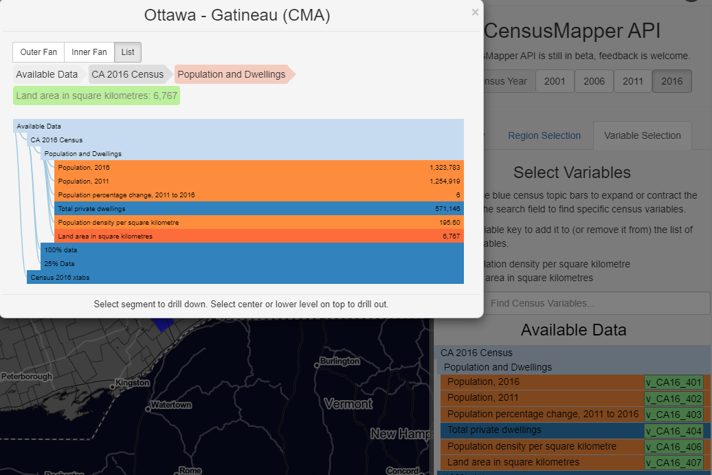
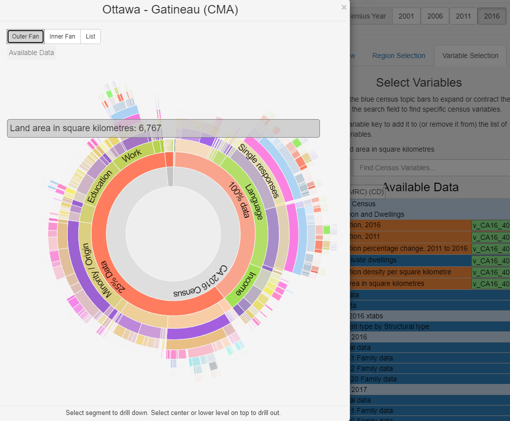
You can discover more census-related data information in the specific region from the [list] section.

You can find census data information which is highly-related to your previous choice in the specific region from [inner fan] section, they are hierarchy relationship from inner to the outer layer.

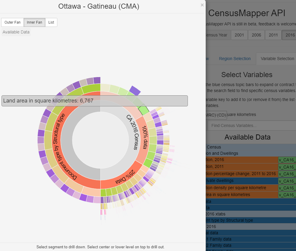
You can discover all census-related data information in the specific region from [outer fan] section, they are hierarchy relationship from inner to the outer layer.

Exprolary Analysis

Notice before downloading Cancensus Package in R

Cancensus provides users with tidy Canadian-census data and useful R functions so that people can manipulate and analyze them. Cancensus is available for R versions above 3.6.4. The easiest way to check your current version is by picking [Global Options] from the [Tools] menu on the top of the R Studio interface.

If your version is lower than 3.6.4, you may use the following code to upgrade:

install.packages(“installr”) library(installr) updateR() ***

Cancensus package in R requires a valid CensusMapper API key to use. If you are planning to download the package and manipulate data, you may go to censusmapper webpage and sign up for a free account at first, you can automatically get your own API_key then add it into options(cancensus.api_key = ““) function.

Moreover, to speed up data manipulation performance and reduce quota usage, it is better to assign a local cache file by using options(cancensus.cache_path = ““) function.

## load your personal API key and cache_path
library(cancensus)
options(cancensus.api_key = "YOUR_API_KEY_GOES_HERE")
options(cancensus.cache_path = "A_SUBDIRECTORY_LOCATION_FOR_SAVING_API_CALLS_SO_YOU_DONT_EXCESSIVELY_REPEAT_THEM")

## Census data is currently stored temporarily.
## 
##  In order to speed up performance, reduce API quota usage, and reduce unnecessary network calls, please set up a persistent cache directory by setting the environment variable CM_CACHE_PATH= '<path to cancensus cache directory>' or  setting options(cancensus.cache_path = '<path to cancensus cache directory>')
## 
##  You may add this environment varianble to your .Renviron or add this option, together with your API key, to your .Rprofile.

Census variable description

Census data contains thousands of geographic regions and dozens of unique variables. The following functions can be used to directly access a proper census dataset so that we can get a proper dataset that includes all available regions and variables in a given year.

## view different regional variables and census variables from 2016 avaiable census datasets
region <- list_census_regions("CA16")
vectors <- list_census_vectors("CA16")

Locating region dataset is aggregated at multiple geographic levels. The following description indicates all available regional names and their codes:

C： Canada
PR： Provinces
CMA：Census Metropolitan Area
CA： Census Agglomeration
CD： Census Division
CSD：Census Subdivision
CT： Census Tracts
DA： Dissemination Area
EA: Enumeration Area (1996 only)
DB: Dissemination Block (2001 - 2016)

For variables dataset, its code and variables descriptions can be organized as follows:

Vector: variable code
Type: aggregates of female, male and total responses
Label: variable name
Units: variable units which include a count integer, percentages and currency figures
Parent_vector: vector code of hierarchical parent category
Aggregation: aggregated methods which include additive and average
Details: summary of short titles

The following secionts of the article is going to subset the original dataset by selecting specific variable topics, such as official language percentage, linear regression of population, and median income data. Then some analysis by plotting basic statistical graphs. More professional examples can be discovered here.

Let’s look for Ottawa in the region variable:

grep(region$name,pattern="Ottawa", value=TRUE)

## [1] "Ottawa - Gatineau" "Ottawa"            "Ottawa"

region[grep(region$name,pattern="Ottawa"),]

## # A tibble: 3 × 8
##   region  name              level     pop municipal_status CMA_UID CD_UID PR_UID
##   <chr>   <chr>             <chr>   <int> <chr>            <chr>   <chr>  <chr> 
## 1 505     Ottawa - Gatineau CMA   1323783 B                <NA>    <NA>   <NA>  
## 2 3506    Ottawa            CD     934243 CDR              <NA>    <NA>   35    
## 3 3506008 Ottawa            CSD    934243 CV               505     3506   35

We can also look for specific terms in the variables dataset

grep(vectors$label,pattern="Education", value=TRUE)

##  [1] "Education"               "Education"              
##  [3] "Education"               "13. Education"          
##  [5] "13. Education"           "13. Education"          
##  [7] "Education"               "Education"              
##  [9] "Education"               "13. Education"          
## [11] "13. Education"           "13. Education"          
## [13] "61 Educational services" "61 Educational services"
## [15] "61 Educational services"

region[grep(vectors$label,pattern="Education"),]

## # A tibble: 15 × 8
##    region  name               level   pop municipal_status CMA_UID CD_UID PR_UID
##    <chr>   <chr>              <chr> <int> <chr>            <chr>   <chr>  <chr> 
##  1 4712031 Tessier            CSD      25 VL               <NA>    4712   47    
##  2 5933836 Lower Hat Creek 2  CSD      25 IRI              <NA>    5933   59    
##  3 1209038 Sheet Harbour 36   CSD      25 IRI              12205   1209   12    
##  4 4713004 Netherhill         CSD      25 VL               <NA>    4713   47    
##  5 5933809 Paul's Basin 2     CSD      25 IRI              <NA>    5933   59    
##  6 5933811 Zoht 4             CSD      25 IRI              <NA>    5933   59    
##  7 5933840 Lytton 4E          CSD       5 IRI              <NA>    5933   59    
##  8 4718062 Missinipe          CSD       5 NH               <NA>    4718   47    
##  9 5941813 Canim Lake 2       CSD       5 IRI              <NA>    5941   59    
## 10 5937805 Harris 3           CSD       5 IRI              <NA>    5937   59    
## 11 6101063 Region 1, Unorgan… CSD       5 NO               <NA>    6101   61    
## 12 2421015 Saint-Louis-de-Go… CSD       5 PE               <NA>    2421   24    
## 13 <NA>    <NA>               <NA>     NA <NA>             <NA>    <NA>   <NA>  
## 14 <NA>    <NA>               <NA>     NA <NA>             <NA>    <NA>   <NA>  
## 15 <NA>    <NA>               <NA>     NA <NA>             <NA>    <NA>   <NA>

Finding variables

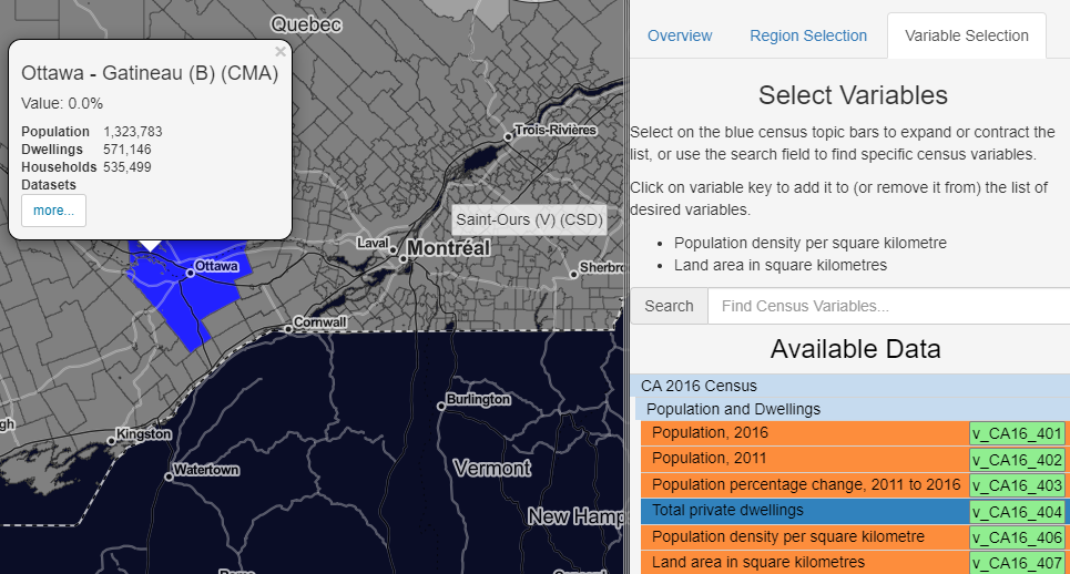
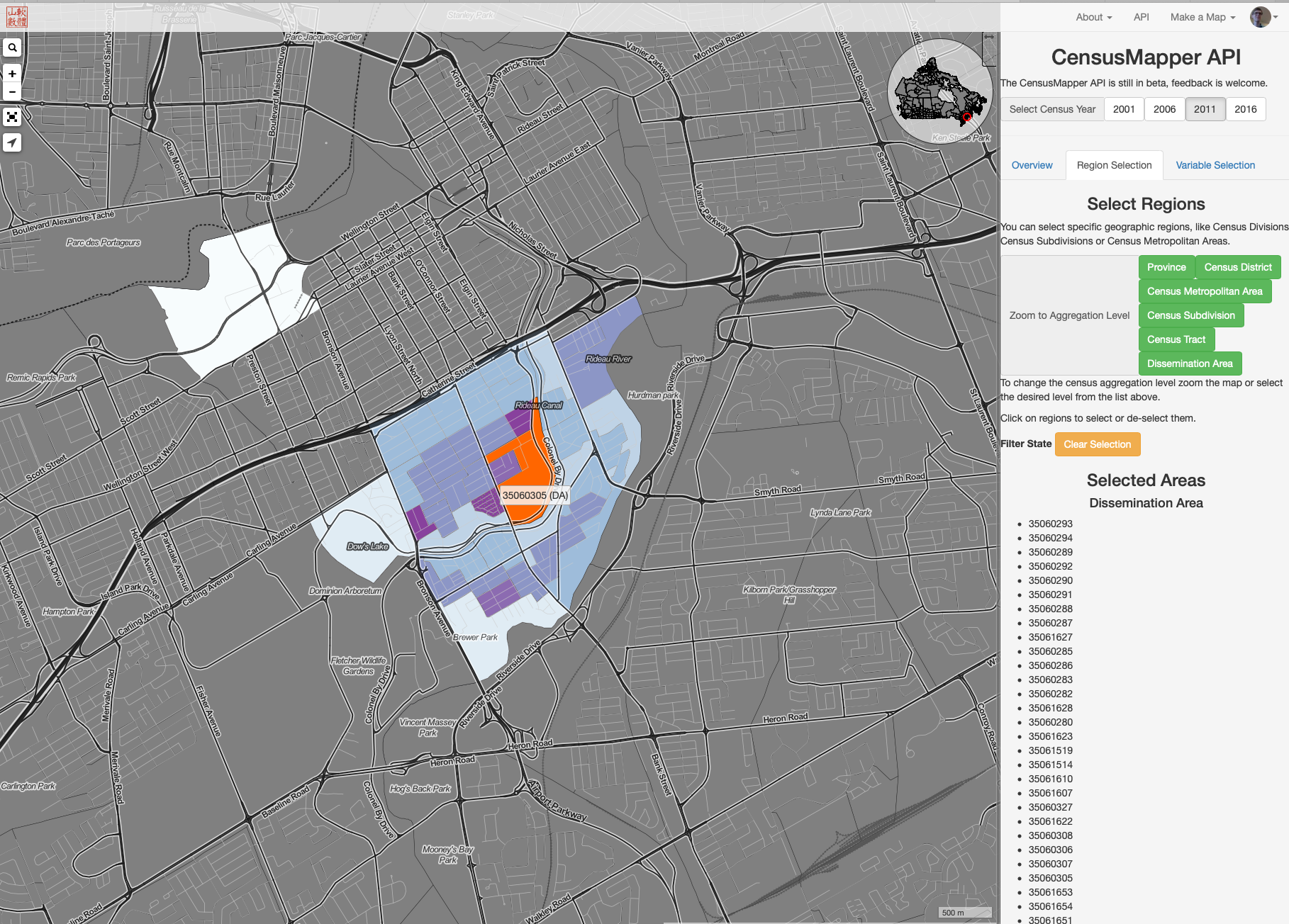
One option is to visit censusmapper.ca, log in and and click on [API]. Click on the census year and select the region(s) you would like. Here I have selected Old Ottawa South.

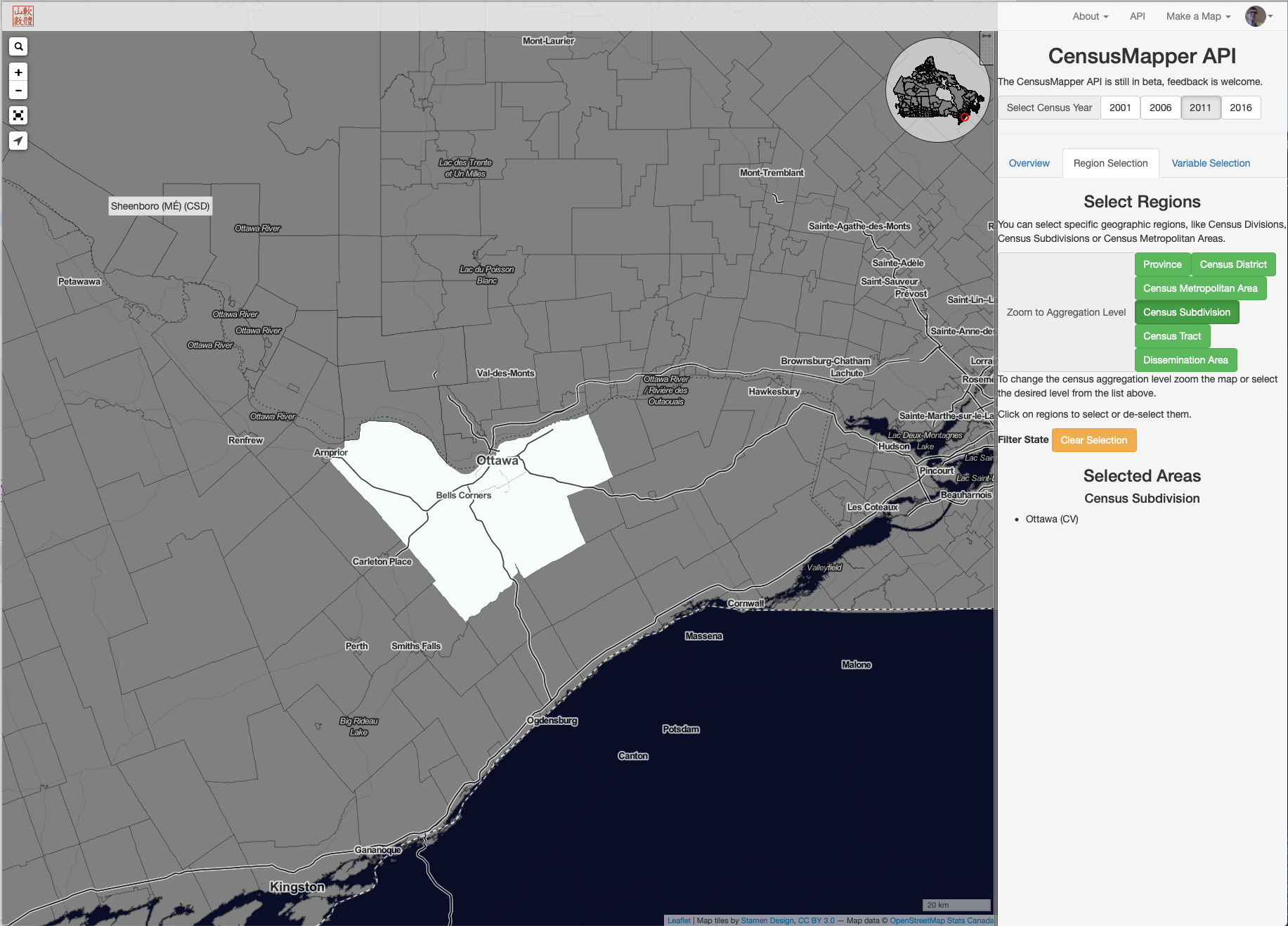
Or you can select the Ottawa Census Subdivision.

Then you switch to the [Variable SElection] tab and dig into the variables of interest. In some cases you can obtain summaries or counts from the full census population. In other cases, to avoid de-annonamyzing the data, only a sample is available.

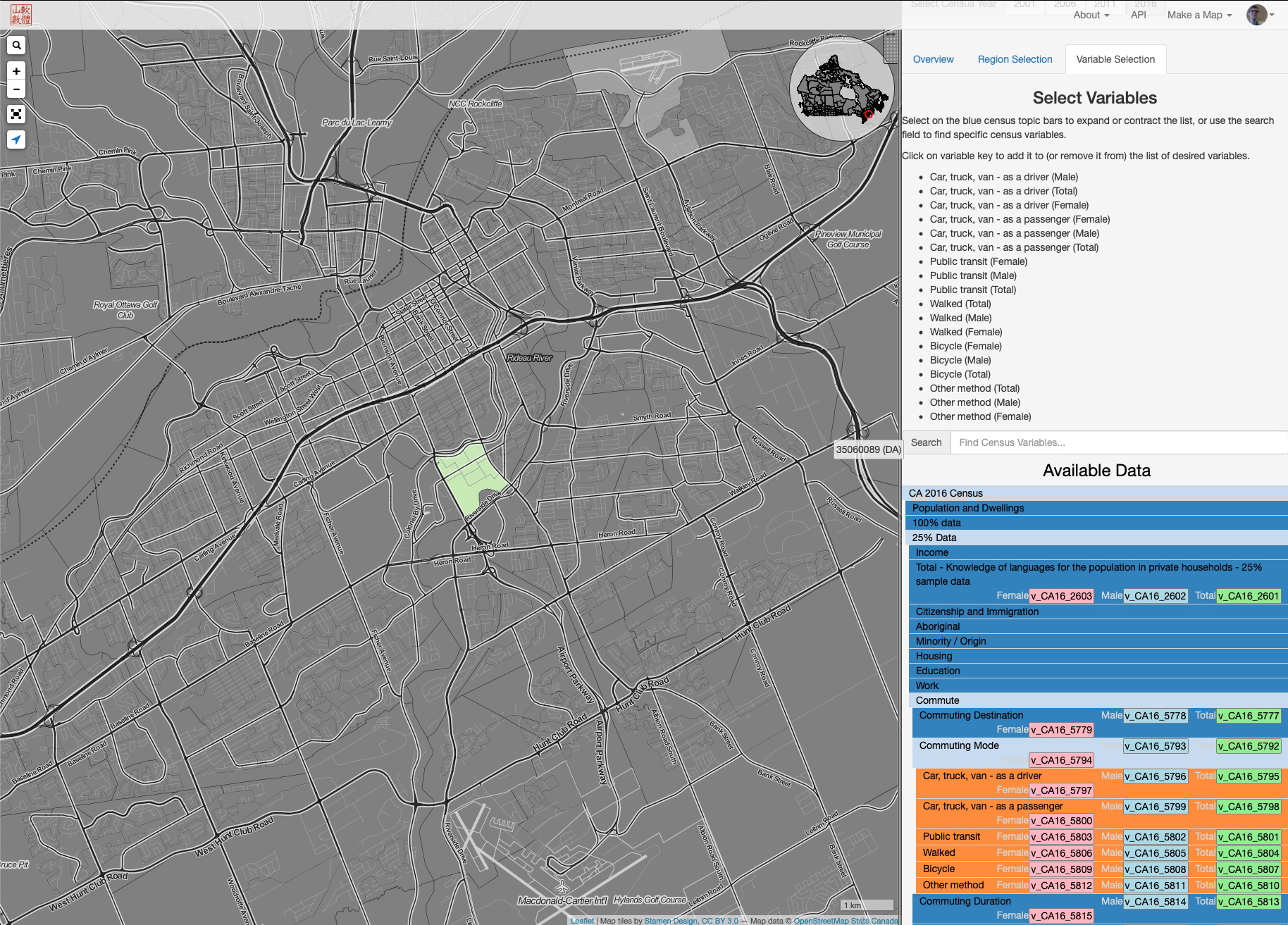
Return to the [Overview] tab and a tthe botom you’ll find code to retrieve your data:

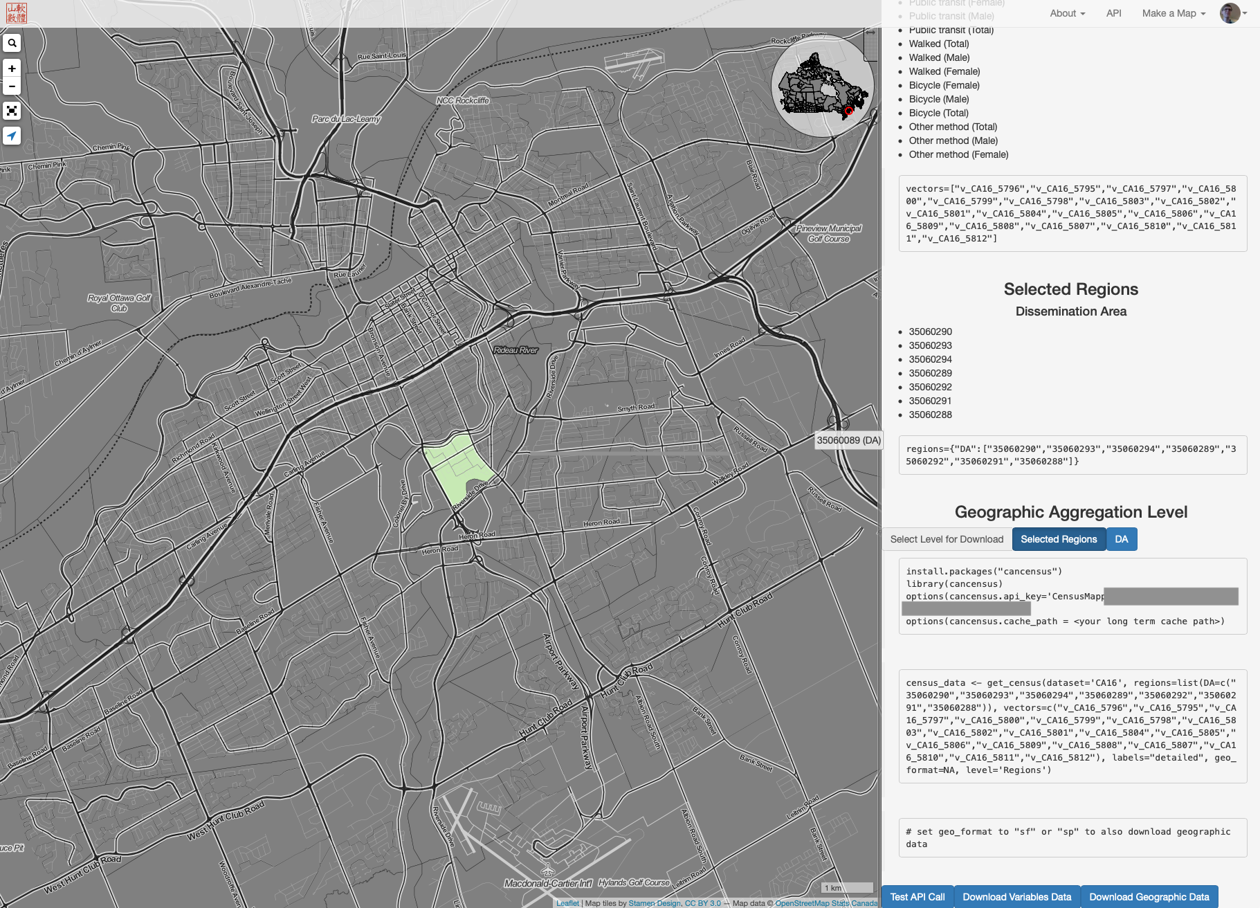
Plugging in the variables and regions we can pull the Census data using the API.

OOS_data <- census_data <- get_census(dataset='CA16', regions=list(DA=c("35060290","35060293","35060294","35060289","35060292","35060291","35060288")), vectors=c("v_CA16_5796","v_CA16_5795","v_CA16_5797","v_CA16_5800","v_CA16_5799","v_CA16_5798","v_CA16_5803","v_CA16_5802","v_CA16_5801","v_CA16_5804","v_CA16_5805","v_CA16_5806","v_CA16_5809","v_CA16_5808","v_CA16_5807","v_CA16_5810","v_CA16_5811","v_CA16_5812"), labels="detailed", geo_format=NA, level='Regions')

## Reading vectors data from local cache.

# or expand out to Ottawa between Bronson and the Rideau and Ottawa Rivers.


Ottawa_data <-  get_census(dataset='CA16', regions=list(DA=
c("35060290","35060293","35060294","35060289","35060292","35060291","35060288","35061627","35060287","35060283","35060285","35060286","35060280","35061628","35060282","35061514","35061607","35061605","35061608","35061610","35061519","35061518","35060307","35060306","35060308","35060327","35061622","35061621","35060366","35060300","35060310","35061653","35060305","35061623","35061654","35060298","35060296","35060297","35060295","35060301","35061651","35061717","35061709","35060314","35060313","35060345","35060346","35060339","35060337","35060367","35060368","35060347","35060315","35061604","35060343","35061710","35061714","35061715","35061713","35061711","35060336","35061705","35061703","35060405","35060330","35060331","35060333","35060334","35061716","35061718","35060329","35060332","35060325","35061511","35060324","35061512","35061510","35061509","35060267","35061780","35061779","35061782","35061778","35061781","35061225","35061783","35060264","35061027","35061799","35061785","35061026","35061787","35061786","35061793","35061791","35061784","35060401","35061602","35061611","35061708","35060312","35061712","35060407","35060406","35060404","35060402","35060408","35060403","35060338","35061788","35061792","35061795","35061796","35061798","35061020","35061797","35061802","35061803","35060255","35061800","35060254","35061789","35060252","35060253","35061790","35060251","35060249","35061794","35061801","35060246","35061222")),
vectors=c("v_CA16_5796","v_CA16_5795","v_CA16_5797","v_CA16_5800","v_CA16_5799","v_CA16_5798","v_CA16_5803","v_CA16_5802","v_CA16_5801","v_CA16_5804","v_CA16_5805","v_CA16_5806","v_CA16_5809","v_CA16_5808","v_CA16_5807","v_CA16_5810","v_CA16_5811","v_CA16_5812"), 
labels="detailed", 
geo_format=NA, 
level='Regions')

## Reading vectors data from local cache.

# or focus on Ottawa between Bronson and the Rideau River and north to Gloucester Street to avoid the working part of downtown.

Ottawa_residential_Urban <- get_census(dataset='CA16', regions=list(DA=c("35060290","35060293","35060294","35060289","35060292","35060291","35060288","35061627","35060287","35060283","35060285","35060286","35060280","35061628","35060282","35061608","35061610","35061519","35061518","35060307","35060306","35060308","35060327","35061622","35061621","35060366","35060300","35060310","35061653","35060305","35061623","35061654","35060298","35060296","35060297","35060295","35060301","35061651","35061717","35061709","35060314","35060313","35060345","35060346","35060339","35060337","35060367","35060368","35060347","35060315","35061604","35060343","35061710","35061714","35061715","35061713","35061711","35060336","35061705","35061703","35060405","35060330","35060331","35060333","35060334","35061716","35061718","35060329","35060332","35060325","35060324","35060401","35061602","35061611","35061708","35060312","35061712","35061514","35061607","35061605")), vectors=c("v_CA16_5796","v_CA16_5795","v_CA16_5797","v_CA16_5800","v_CA16_5799","v_CA16_5798","v_CA16_5803","v_CA16_5802","v_CA16_5801","v_CA16_5804","v_CA16_5805","v_CA16_5806","v_CA16_5809","v_CA16_5808","v_CA16_5807","v_CA16_5810","v_CA16_5811","v_CA16_5812","v_CA16_4964","v_CA16_4965","v_CA16_4963","v_CA16_1","v_CA16_2","v_CA16_3"), labels="detailed", geo_format=NA, level='Regions')

## Reading vectors data from local cache.

Select your final data set and we can make new variables and look at some data.

data2use = Ottawa_residential_Urban

#Format the column nammes by removing spaces and replacing punctuation with "."

colnames(data2use) =  gsub(colnames(data2use),pattern="\\s|[[:punct:]]",replacement = ".")

data2use = data2use  |> rename(v.CA16.5805..Walked.Male   = v.CA16.5805..Walked, 
                     v.CA16.5806..Walked.Female = v.CA16.5806..Walked,
                     v.CA16.5806..Walked.Total  = v.CA16.5804..Walked,
                     v.CA16.4963..Average.after.tax.income.in.2015.among.recipients....Total  = v.CA16.4963..Average.after.tax.income.in.2015.among.recipients....,
                     v.CA16.4964..Average.after.tax.income.in.2015.among.recipients....Male  = v.CA16.4964..Average.after.tax.income.in.2015.among.recipients....,
                     v.CA16.4965..Average.after.tax.income.in.2015.among.recipients....Female  = v.CA16.4965..Average.after.tax.income.in.2015.among.recipients....)|>
  mutate(People_per_sqkm = Population / Area..sq.km., 
        Proportion_walked = v.CA16.5806..Walked.Total/Population) 




data2use |>
ggplot(aes(x = v.CA16.4965..Average.after.tax.income.in.2015.among.recipients....Female, y= v.CA16.4964..Average.after.tax.income.in.2015.among.recipients....Male))+
  geom_point()+
   labs(y = "Average Income for Males",x = "Average Income for Females") +
  ggtitle("Comparing Income In the Urban Core of Ottawa")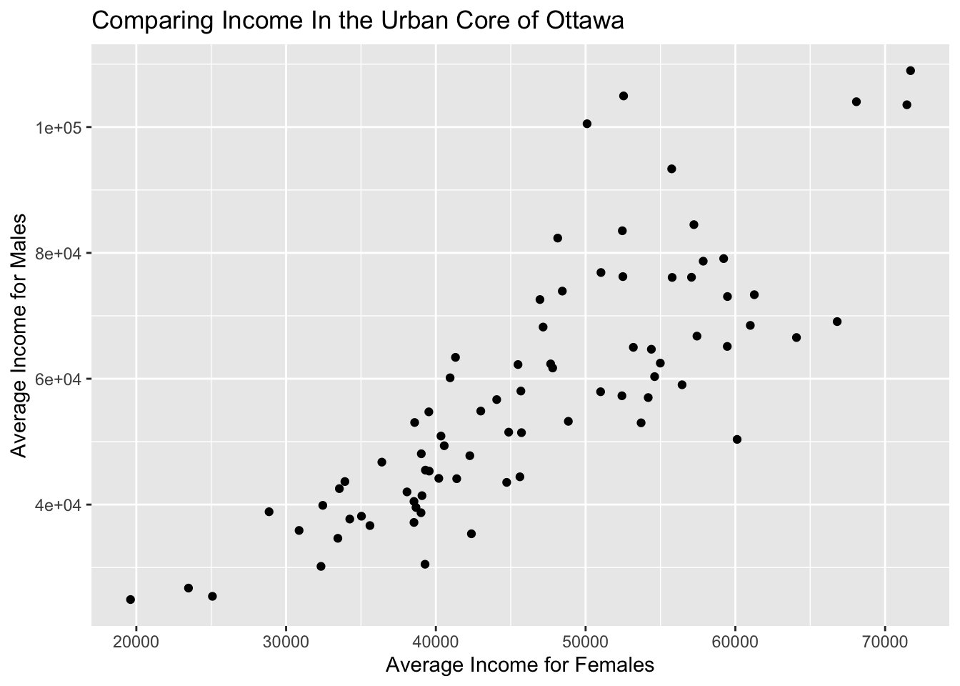

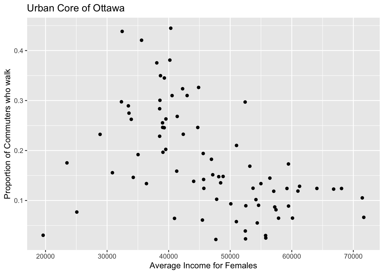
data2use |>
ggplot(aes(x = v.CA16.4965..Average.after.tax.income.in.2015.among.recipients....Female, 
           y= Proportion_walked))+
  geom_point()+
   labs(y = "Proportion of Commuters who walk",x = "Average Income for Females") +
  ggtitle("Urban Core of Ottawa")

Census Data: Census Mapper - CensusMapper and Statistics Canada