Unit 12
Last week, we mentioned that the Maximum-Cardinality Stable Set Problem is \(\mathcal{NP}\)-hard. But what exactly does that mean?
We will not try to define \(\mathcal{NP}\)-hardness. The Wikipedia has an article on the topic. The topic is also covered in MATH 3804. If you are interested in reading more about the topic, see some of the following resources:
A couple of videos on the P vs. NP problme are:
For the purpose of these notes, all we need to know is that if a problem is \(\mathcal{NP}\)-hard, there is no known algorithm that runs in time polynomial in the size of the problem instance. A proper definition requires one to specify exactly what is meant by an algorithm and how to measure the size of a problem instance.
Many combinatorial optimization problems encountered in practice are \(\mathcal{NP}\)-hard. Even though there do not yet exist polynomial-time algorithms to solve these problems exactly, there do exist polynomial-time algorithms that return near-optimal solutions with some sort of guarantee for some of these problems. For instance, there might be \(\alpha\)-approximation algorithms for a minimization problem that obtains a solution with objective function value no greater than \(\alpha\) times the optimal value in polynomial time. Hence, the objective function value of the returned solution could be anywhere between the optimal value and \(\alpha\) times the optimal value.
Recall that given an undirected graph \(G = (V,E)\), a node cover is a subset \(C \subseteq V\) such that every edge in \(E\) has an end in \(C\). The Minimum-Cardinality Node Cover Problem is to find a node cover of minimum cardinality.
In the case when \(G\) is bipartite, we have already seen how to obtain a minimum-cardinality node cover in our discussion of maximum-cardinality matching for bipartite graphs. Nevertheless, the Minimum-Cardinality Node Cover Problem is \(\mathcal{NP}\)-hard. We will look at two \(2\)-approximation algorithms for the problem.
Algorithm 12.1.
Input: An undirected graph \(G = (V,E)\)
Output: A node cover \(C\)
\(C \leftarrow \emptyset\)
while \(E \neq \emptyset\)
choose any \(uw \in E\)
\(C \leftarrow C \cup \{u,w\}\)
remove from \(E\) all the edges that are incident to \(u\) or \(w\)
return \(C\)
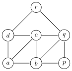
We apply Algorithm 12.1 to the graph depicted below:
Initially, \(C = \emptyset\) and \(E = \{ab, ac, ad, bc, bp, bq, cd, cq, dr, pq, qr\}\).
Suppose that the edge \(cd\) is chosen in step 2.A. The nodes \(c\) and \(d\) are added to \(C\) and all the edges with \(c\) or \(d\) as an endnode are removed from \(E\). Hence, \(C = \{c,d\}\) and \(E = \{ab, bp, bq, pq, qr\}\).
Next, suppose that the edge \(bq\) is chosen in step 2.A. The nodes \(b\) and \(q\) are added to \(C\) and all the edges with \(b\) or \(q\) as an endnode are removed from \(E\). Hence, \(C = \{b,c,d,q\}\) and \(E = \emptyset\). Since \(E = \emptyset\), the algorithm stops and returns the node cover \(C = \{b,c,d,q\}\) which turns out to be optimal.
The second algorithm works with the following linear programming relaxation known as the fractional node cover problem: \[\begin{array}{rll} \min & \displaystyle\sum_{v \in V} x_v \\ (FNC)~~~~\text{s.t.} & x_u + x_w \geq 1 & \forall~uw \in E \\ & x_u \geq 0 & \forall~u \in V \end{array}\]
Proposition 12.1. In every extreme-point solution of \((FNC)\), each of its entries is \(0\), \(\frac{1}{2}\), or \(1\).
Proof. (Sketch) Suppose \(\mathbf{x}^*\) is a feasible solution to \((FNC)\) that has at least one entry that is not equal to \(0\), \(\frac{1}{2}\), or \(1\).
Let \(R = \{ v \in V : 0 < x^*_v < \frac{1}{2}\}\).
Let \(S = \{ v \in V : \frac{1}{2} < x^*_v < 1\}\).
Let \(\epsilon > 0\) be such that \(\epsilon < x^*_v < \frac{1}{2}-\epsilon\) for all \(v \in R\) and \(\frac{1}{2}+\epsilon < x^*_v < 1-\epsilon\) for all \(v \in S\).
Let \(\mathbf{x}'\) be \(\mathbf{x}^* + \epsilon \chi^R - \epsilon \chi^S\). Let \(\mathbf{x}''\) be \(\mathbf{x}^* - \epsilon \chi^R + \epsilon \chi^S\). Note that \(\mathbf{x}'\neq \mathbf{x}''\).
It can be checked that \(\mathbf{x}'\) and \(\mathbf{x}''\) are feasible solutions to \((FNC)\). Since \(\mathbf{x}^* = \frac{1}{2}\mathbf{x}' + \frac{1}{2}\mathbf{x}''\), \(\mathbf{x}^*\) is not an extreme-point solution.
Algorithm 12.2.
Input: An undirected graph \(G = (V,E)\)
Output: A node cover \(C\)
obtain an extreme-point optimal solution \(\mathbf{x}^*\) to \((FNC)\)
\(C \leftarrow \{ v \in V : x^*_v > 0 \}\)
return \(C\)
Let \(\nu\) denote the minimum cardinality of a node cover. Let \(\nu^*\) denote the optimal value of \((FNC)\). Note that \(\chi^C \geq \mathbf{x}^*\). Hence, \(\chi^C\) is a feasible solution to \((FNC)\). Now, \(x^*_v\) is at least \(\frac{1}{2}\) for all \(v\) such that \(x^*_v > 0\). Hence, for all \(v\) with \(x^*_v > 0\), we have \(2x^*_v \geq 1 = \chi^C_v\). Thus, \(|C| = \sum_{v \in V} \chi^C_v \leq \sum_{v \in V} 2x^*_v = 2\nu^*\). Since \(\nu^* \leq \nu\), we have that \(|C| \leq 2\nu\).
Observe that the previous argument actually shows that \(|C|\) is at most twice the optimal value of \((FNC)\). Thus, \(\nu^* \leq \nu \leq |C| \leq 2\nu^*\). In other words, the minimum cardinality of a node cover is at most \(2\) times the optimal value of the linear programming relaxation \((FNC)\). We call the factor \(2\) the integrality gap of \((FNC)\) for the Minimum-Cardinality Node Cover Problem. Recently, Mohit Singh (2019) showed that the integrality gap of \((FNC)\) can be improved to \(2-\frac{2}{\chi^f(G)}\) where \(\chi^f(G)\) is the fractional chromatic number of \(G\) defined as the optimal value of \[\begin{array}{rll} \min & \displaystyle\sum_{S \in \mathcal{S}} x_S \\ \text{s.t.} & \displaystyle\sum_{S \in \mathcal{S}\;:\;u \in S} x_S \geq 1 & \forall~u \in V \\ & x_S \geq 0 & \forall~S \in \mathcal{S}. \end{array}\] where \(\mathcal{S}\) denotes the set of stable sets in \(G\).
We apply Algorithm 12.2 to the graph in the example above. For this graph, \((FNC)\) is \[\begin{array}{rll} \min & x_a + x_b + x_c + x_d + x_p + x_q + x_r \\ \text{s.t.} & x_a + x_b >= 1 \\ & x_a + x_c >= 1 \\ & x_a + x_d >= 1 \\ & x_b + x_c >= 1 \\ & x_b + x_p >= 1 \\ & x_b + x_q >= 1 \\ & x_c + x_d >= 1 \\ & x_c + x_q >= 1 \\ & x_d + x_r >= 1 \\ & x_p + x_q >= 1 \\ & x_q + x_r >= 1 \\ & x_a, x_b, x_c, x_d, x_p, x_q, x_r \geq 0. \end{array}\] An extreme-point optimal solution is \(x^*_a = x^*_b = x^*_c = x^*_d = x^*_p = x^*_q = x^*_r = \frac{1}{2}.\) Hence, \(C = \{a,b,c,d,p,q,r\}\) with cardinality 7, which is still no more than twice the minimum value of a node cover. Note that this solution is far worse than the one obtained by Algorihtm 12.1. However, it is not necessarily true that one algorithm will always perform better than the other.
The Travelling Salesman Problem (TSP) is probably the most studied \(\mathcal{NP}\)-hard problem in combinatorial optimization.
Given a complete graph Let \(G=(V,E)\) be a complete graph. That is, \(uv \in E\) for all distinct \(u,v \in V\). The edge costs are given by \(\mathbf{c} \in \mathbb{R}^E\). We call a cycle in \(G\) hamiltonian if it has exactly \(|V|\) edges. The TSP is the problem of finding a minimum-cost hamiltonian cycle.
An integer-programming formulation due to Dantzig, Fulkerson, and Johnson (1954) is \[\begin{array}{rll} \min & \displaystyle\sum_{e \in E} c_e x_e \\ (TSP)~~~\text{s.t.} & \mathbf{x}(\delta(v)) = 2 & \forall~v \in V\\ & \mathbf{x}(\delta(S)) \geq 2 & \forall~S \subset V,~\emptyset \neq S \neq V\\ & \mathbf{x} \geq \mathbf{0} \\ & \mathbf{x} \in \mathbb{Z}^E. \end{array}\]
The TSP has often been studied under the assumption that \[c_{uw} + c_{wv} \geq c_{uv}\] for all distinct \(u,v,w \in V\). Under this assumption Christofides Algorithm returns in polynomial time a hamiltonion cycle with cost no more than \(\frac{3}{2}\) of the optimal cost. A recently-announced result gave a slight improvement.
Removing the integrality constraints from \((TSP)\) gives what is known as the Dantzig-Fulkerson-Johnson relaxation of the TSP. Under the same assumption on \(\mathbf{c}\), Held and Karp (1970) showed that the optimal cost of a hamiltonion cycle is at most \(\frac{3}{2}\) times the optimal value of the LP relaxation. However, it is not known if \(\frac{3}{2}\) is the best possible. In fact, Goemans (1995) conjectured that the optimal cost of a hamiltonion cycle is at most \(\frac{4}{3}\) times the optimal value of the LP relaxation. As of 2020, the conjecture is still open.
For more on the TSP, visit http://www.math.uwaterloo.ca/tsp/.
Let \(G = (V, E)\) denote the undirected graph depicted below:
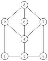
Is there a node cover having cardinality 3?
Show that Algorithm 12.1 could choose the following edges in step 2.A in the order shown: \(\{1,2\}\), \(\{3,4\}\), \(\{5,7\}\), \(\{6,8\}\), thus giving the node cover \(C\) consisting of all the nodes.
Is there an execution of Algorithm 12.1 that returns a node cover of cardinality at most 6.
Write down the linear programming problem that solves the fractional node cover problem for \(G\).
Recall that the fractional chromatic number of \(G\) is defined as the optimal value of the LP problem \[\begin{array}{rll} \min & \displaystyle\sum_{S \in \mathcal{S}} x_S \\ \text{s.t.} & \displaystyle\sum_{S \in \mathcal{S}\;:\;u \in S} x_S \geq 1 & \forall~u \in V \\ & x_S \geq 0 & \forall~S \in \mathcal{S} \end{array}\] where \(\mathcal{S}\) denotes the set of stable sets in \(G\).
Show that \(\mathcal{S}\) may be replaced with the set of maximal stable sets. (A stable set is maximal if it is not properly contained in another stable set.)
Write down the LP for the graph \(G\) above where \(\mathcal{S}\) is the set of maximal stable sets.
No. It is because \(\{\{1,3\}, \{5,7\}, \{4,6\}, \{2,8\}\}\) is a matching of cardinality four and the cardinality of a node cover cannot be less than the cardinality of a matching in the same graph.
The algorithm can have the following iterations:
Iteration 1.
In step 2.A., we can choose \(\{1,2\}\).
After step 2.B. and 2.C, we have \(C = \{1,2\}\) and \(E = \{\{3,4\}, \{3,5\}, \{4,6\}, \{4,7\}, \{5,7\}, \{6,7\}, \{6,8\}, \{7,8\}\}.\)
Iteration 2.
In step 2.A., we can choose \(\{3,4\}\) since it is in \(E\).
After step 2.B. and 2.C, we have \(C = \{1,2,3,4\}\) and \(E = \{\{5,7\},\{6,7\},\{6,8\},\{7,8\}\}.\)
Iteration 3.
In step 2.A., we can choose \(\{5,7\}\) since it is in \(E\).
After step 2.B. and 2.C, we have \(C = \{1,2,3,4,5,7\}\) and \(E = \{\{6,8\}.\)
Iteration 4.
In step 2.A., we can choose \(\{6,8\}\) since it is in \(E\).
After step 2.B. and 2.C, we have \(C = \{1,2,3,4,5,6,7,8\}\) and \(E = \emptyset.\)
Since \(E\) is now empty, the algorithm returns \(C\) which consists of all the nodes of \(G\).
See the following:
Iteration 1.
In step 2.A., we can choose \(\{6,8\}\).
After step 2.B. and 2.C, we have \(C = \{6,8\}\) and \(E = \{\{1,2\},\{1,3\},\{2,4\}, \{3,4\},\{3,5\},\{4,7\},\{5,7\}\}.\)
Iteration 2.
In step 2.A., we can choose \(\{2,4\) since it is in \(E\).
After step 2.B. and 2.C, we have \(C = \{2,4,6,8\}\) and \(E = \{\{1,3\},\{3,5\},\{5,7\}\}.\)
Iteration 3.
In step 2.A., we can choose \(\{3,5\}\) since it is in \(E\).
After step 2.B. and 2.C, we have \(C = \{2,3,4,5,6,8\}\) and \(E = \emptyset.\)
Since \(E\) is now empty, the algorithm returns \(C\).
The LP is \[\begin{array}{rll} \min & x_1 + x_2 + x_3 + x_4 + x_5 + x_6 + x_7 + x_8 \\ \text{s.t.} & x_1 + x_2 \geq 1 \\ & x_1 + x_3 \geq 1 \\ & x_2 + x_4 \geq 1 \\ & x_2 + x_6 \geq 1 \\ & x_2 + x_8 \geq 1 \\ & x_3 + x_4 \geq 1 \\ & x_3 + x_5 \geq 1 \\ & x_4 + x_6 \geq 1 \\ & x_4 + x_7 \geq 1 \\ & x_5 + x_7 \geq 1 \\ & x_6 + x_7 \geq 1 \\ & x_6 + x_8 \geq 1 \\ & x_7 + x_8 \geq 1 \\ & x_1, x_2, x_3, x_4, x_5, x_6, x_7, x_8 \geq 0. \end{array}\] Here, \(x_{i}\) is the variable corresponding to the node \(i\).
To see that considering maximal sets suffices, let \(S_1\) and \(S_2\) be stable sets with \(S_1 \subsetneq S_2\) and \(x^*\) be a feasible solution to the LP problem. Note that we can transfer the value of \(x_{S_1}\) to \(x_{S_2}\) without affecting feasibility and the objective function value.
For the given \(G\), the maximal stable sets are \(\{1,7\}\), \(\{1,4,5,8\}\), \(\{1,5,6\}\), \(\{2,3,7\}\), \(\{25\}\), \(\{3,6\}\), and \(\{3,8\}\). Hence, the LP is \[\begin{array}{rll} \min & x_{\{1,7\}} + x_{\{1,4,5,8\}} + x_{\{1,5,6\}} + x_{\{2,3,7\}} + x_{\{2,5\}} + x_{\{3,6\}} + x_{\{3,8\}} \\ \text{s.t.} & x_{\{1,7\}} + x_{\{1,4,5,8\}} + x_{\{1,5,6\}} \geq 1 \\ & x_{\{2,3,7\}} + x_{\{2,5\}} \geq 1 \\ & x_{\{2,3,7\}} + x_{\{3,6\}} + x_{\{3,8\}} \geq 1 \\ & x_{\{1,4,5,8\}} \geq 1 \\ & x_{\{1,4,5,8\}} + x_{\{1,5,6\}} + x_{\{2,5\}} \geq 1 \\ & x_{\{1,5,6\}} + x_{\{3,6\}} \geq 1 \\ & x_{\{1,7\}} + x_{\{2,3,7\}} \geq 1 \\ & x_{\{1,4,5,8\}} + x_{\{3,8\}} \geq 1 \\ & x_{\{1,7\}}, x_{\{1,4,5,8\}}, x_{\{1,5,6\}}, x_{\{2,3,7\}}, x_{\{2,5\}}, x_{\{3,6\}}, x_{\{3,8\}} \geq 0. \end{array}\]